If you are a data scientist, data analysts, product manager in a data-driven company, you experiment with your product a lot, and usually you do lots of AB tests.
Let’s assume you have an AB test with control and treatment groups. When analysing results, you compare the average number of orders/visits/views (or any other metric) in test groups. Obviously, you can calculate the mean of a metric, you can even say using t-test and p-value if there is statistically significant difference between two means. But usually, they say don’t look only at p-values, look at confidence intervals.
In this blog post, we discover how to calculate confidence intervals using bootstrapping. Bootstrapping is a cool method to estimate confidence intervals because it does not rely on any assumption of data distribution (compared to popular Welch t-test, for example) and it is quite easy to implement by yourself (I share a link to my implementation below).
Bootstrap definition and principle
The bootstrap is a method for estimating standard errors and computing confidence intervals. Bootstrapping started in 1970th by Bradley Efron; it has already existed for more than 40 years, so many different types and methods of bootstrapping were developed since then.
But despite of many variations, all bootstrap steps look as follows:
- Obtain data sample x1,x2,…,xn drawn from a distribution F.
- Define u – statistic computed from the sample (mean, median, etc).
- Sample x*1, x*2, . . . , x*n with replacement from the original data sample. Let it be F* – the empirical distribution. Repeat n times (n is bootstrap iterations).
- Compute u* – the statistic calculated from each resample.
Then the bootstrap principle says that:
- Empirical distribution from bootstraps is approximately equal to distribution of sample data: F* ≈ F.
- The variation of statistic computed from the sample u is well-approximated by the variation of statistic computed from each resample u*. So, computed statistic u* from bootstrapping is a good proxy for statistic of sample data.
As mentioned, bootstrap can be applied for different goals:
- Estimating Confidence intervals
- Hypothesis testing
- Bias elimination
Each topic deserves a separate post and today we concentrate only on bootstrapping confidence intervals.
Methods for Bootstrapping Confidence Intervals
When I researched the topic, I haven’t found a single source with all bootstraps methods at once, every reference has its own types. Most common ones are presented below:
- Empirical Bootstrapping
In a nutshell, this method approximates the difference between bootstrapped means and sample mean.
Let’s consider an example (it will continue for other methods as well): estimate the mean μ of the underlying distribution and give an 80% bootstrap confidence interval.
Empirical bootstrapping says:
- Start with resampling with replacement from original data n times.
- For each bootstrap calculate mean x*.
- Compute δ* = x* − x for each bootstrap sample (x is mean of original data), sort them from smallest to biggest.
- Choose δ.1 as the 90th percentile, δ.9 as the 10th percentile of sorted list of δ*, which gives an 80% confidence interval of [x−δ.1, x−δ.9].
Wasserman’s “All of Statistics” book provides with the following math notation for empirical bootstrap:

where x is mean of original data and x* is bootstrap means.
2. Percentile bootstrap
Instead of computing the differences δ*, the bootstrap percentile method uses the distribution of the bootstrap sample statistic as a direct approximation of the data sample statistic.
For Percentile bootstrap:
- Start with resampling with replacement from original data n times.
- For each bootstrap calculate mean x*, sort them from smallest to biggest.
- Choose x*.1 as the 10th percentile, x*.9 as the 90th percentile of sorted list of x*, which gives an 80% confidence interval of [x*.1, x*.9].
Or, in other words:

The bootstrap percentile method is quite simple, but it depends on the bootstrap distribution of x* based on a particular sample being a good approximation to the true distribution of x (because of that reason, this source advises not to use percentile bootstrap).
3. Normal bootstrap
Instead of taking percentiles of bootstrapped means, normal bootstrap method calculates confidence intervals for these bootstrapped means.
- Start with resampling with replacement from original data n times.
- For each bootstrap calculate mean x*.
- Calculate 80% confidence intervals for array of x* using for example, Student t-test:
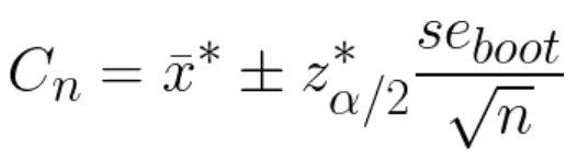
where x* is the sample mean from bootstrap means, se is the standard error of the bootstrap means, z* is critical value (found from the distribution table of normal CDF).
When I compared this method to others, its CI were always very narrow compared to other methods which puzzled me a lot. As I understood, it is because the definition strongly relies on assumption about normal distribution of data.
Some time later, I stumbled upon slightly different wording of this method in Wasserman’s “All of Statistics”. Calculation differs by just one parameter, but it gives a huge difference.
4. Normal interval bootstrap
Normal interval bootstrap repeats all steps of normal bootstrap, but use the following formula for CI:
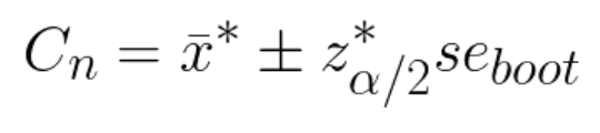
where se_boot is the bootstrap estimate of the standard error.
This interval is not accurate unless the distribution of x* is close to Normal.
Basically, here formula has no division by squared root of n. I haven’t found explanation why it is done in that way. If you have any ideas, please, share them in comments.
5. Parametric Bootstrap
Parametric bootstrap is very close to empirical approach, the only difference is in the source of the bootstrap sample. For the parametric bootstrap, we generate the bootstrap sample from a parametrized distribution. It is often used for the efficient computation of Bayes posterior distributions, not for experimentation analysis, so I will not go into its details here.
Comparing methods
As promised earlier, here you can find Python implementation of all methods. The goal was to estimate 95% bootstrap confidence interval for the mean of target metric. I played with bootstrap methods, number of bootstrap samples and sample size of data itself.
The main question I had: which bootstrap method would show more reliable results. First of all, normal bootstrap crearly produces too narrow CI (because of normality assumptions). Other 3 methods are usually close to each other given large enough sample. The advantage of percentile and empirical types is that they provide different intervals from left and right sides (in contrast to normal interval bootstrap). Usually, it is better because it accounts for distribution of data. As you can see on plot below, intervals for percentile and empirical bootstraps are greeter from the left side – on the side where population mean lies.

[“ci” is confidence intervals for sample data estimated with student t-test]
Choosing between percentile and empirical methods, I am more inclined towards the percentile approach because of its simplicity. Its results are very close to the empirical method, and at the same time requires one step less in calculations.
Another important question: how many bootstrap samplings to do. It depends on data size. If there are less than 1000 data points, it is reasonable to take bootstrap number no more than twice less data size (if there are 400 samples, use no more than 200 bootstraps – further increase doesn’t provide any improvements). If you have more data, the number of bootstraps between 100 and 500 is sufficient (higher number usually will not increase accuracy of CI).
Instead of conclusion
One critical remark one should remember using bootstrapping is that it can’t improve point estimate, meaning the quality of bootstrapping depends on the quality of collected data. If sample data is biased and doesn’t represent population data well, the same will occur with bootstrap estimates. So, always keep in mind that data collected during experimentation should be a good approximation of the whole population data.
In this blog post, I described and compared basic bootstrap methods. Actually, there exist many more methods (like Poisson, Gaussian, Block, etc). Also, bootstrap is not only about confidence intervals, it is used for estimation of standard error of the median, 75% percentiles, hypothesis testing, etc. All of them are good topics for next blog posts 🙂