Recently, I finished the Stanford course CS224W Machine Learning with Graphs. This is Part 2 of blog posts series where I share my notes from watching lectures. The rest you can find here: 1, 3, 4.

Lecture 6 – Message Passing and Node Classification

Slides, Video

Node classification means: given a network with labels on some nodes, assign labels to all other nodes in the network. The main idea for this lecture is to look at collective classification leveraging existing correlations in networks.

Individual behaviors are correlated in a network environment. For example, the network where nodes are people, edges are friendship, and the color of nodes is a race: people are segregated by race due to homophily (the tendency of individuals to associate and bond with similar others).

“Guilt-by-association” principle: similar nodes are typically close together or directly connected; if I am connected to a node with label X, then I am likely to have label X as well.

Collective classification

Intuition behind this method: simultaneously classify interlinked nodes using correlations.

Applications of the method are found in:

document classification,
speech tagging,
link prediction,
optical character recognition,
image/3D data segmentation,
entity resolution in sensor networks,
spam and fraud detection.

Collective classification is based on Markov Assumption – the label Y_i of one node i depends on the labels of its neighbours N_i:

$P(Y_i|i)=P(Y_i|N_i)$

Steps of collective classification algorithms:

Local Classifier: used for initial label assignment.
- Predict label based on node attributes/features.
- Standard classification task.
- Don’t use network information.
Relational Classifier: capture correlations between nodes based on the network.
- Learn a classifier to label one node based on the labels and/or attributes of its neighbors.
- Network information is used.
Collective Inference: propagate the correlation through the network.
- Apply relational classifier to each node iteratively.
- Iterate until the inconsistency between neighboring labels is minimized.
- Network structure substantially affects the final prediction.

If we represent every node as a discrete random variable with a joint mass function p of its class membership, the marginal distribution of a node is the summation of p over all the other nodes. The exact solution takes exponential time in the number of nodes, therefore they use inference techniques that approximate the solution by narrowing the scope of the propagation (e.g., only neighbors) and the number of variables by means of aggregation.

Techniques for approximate inference (all are iterative algorithms):

Relational classifiers (weighted average of neighborhood properties, cannot take node attributes while labeling).
Iterative classification (update each node’s label using own and neighbor’s labels, can consider node attributes while labeling).
Belief propagation (Message passing to update each node’s belief of itself based on neighbors’ beliefs).

Probabilistic Relational classifier

The idea is that class probability of Y_i is a weighted average of class probabilities of its neighbors.

For labeled nodes, initialize with ground-truth Y labels.
For unlabeled nodes, initialize Y uniformly.
Update all nodes in a random order until convergence or until maximum number of iterations is reached.

Repeat for each node i and label c:

$P(Y_i=c)=\frac{1}{\sum_{(i,j)}^{} W(i,j)} \sum_{(i,j \in E)}^{} W(i,j) P(Y_i=c)$

W(i,j) is the edge strength from i to j.

Example of 1^st iteration for one node:

Challenges:

Convergence is not guaranteed.
Model cannot use node feature information.

Iterative classification

Main idea of iterative classification is to classify node i based on its attributes as well as labels of neighbour set N_i:

Architecture of iterative classifier:

Bootstrap phase:
- Convert each node i to a flat vector a_i (Node may have various numbers of neighbours, so we can aggregate using: count , mode, proportion, mean, exists, etc.)
- Use local classifier f(a_i) (e.g., SVM, kNN, …) to compute best value for Y_i .
Iteration phase: iterate till convergence. Repeat for each node i:
- Update node vector a_i.
- Update label Y_i to f(a_i).
- Iterate until class labels stabilize or max number of iterations is reached.

Note: Convergence is not guaranteed (need to run for max number of iterations).

Application of iterative classification:

REV2: Fraudulent User Predictions in Rating Platforms [Kumar et al.]. The model uses fairness, goodness and reliability scores to find malicious apps and users who give fake ratings.

Loopy belief propagation

Belief Propagation is a dynamic programming approach to answering conditional probability queries in a graphical model. It is an iterative process in which neighbor variables “talk” to each other, passing messages.

In a nutshell, it works as follows: variable X₁ believes variable X₂ belongs in these states with various likelihood. When consensus is reached, calculate final belief.

Message passing:

Task: Count the number of nodes in a graph.
Condition: Each node can only interact (pass message) with its neighbors.
Solution: Each node listens to the message from its neighbor, updates it, and passes it forward.

Loopy belief propagation algorithm:

Initialize all messages to 1. Then repeat for each node:

$m_{i\rightarrow j}(Y_i) = \alpha \sum _{Y_i \in \Lambda }{\psi (Y_i,Y_j) } \phi_i (Y_i)\prod_{k \in N_i /j}{m_k \rightarrow j}(Y_i)$

Label-label potential matrix ψ: dependency between a node and its neighbour. ψ(Y_i , Y_j) equals the probability of a node j being in state Y_j given that it has a i neighbour in state Y_i .
Prior belief ϕ_i: probability ϕ_i(Y_i) of node i being in state Y_i.
m(i->j)(Y_i) is i’s estimate of j being in state Y_j.
Λ is the set of all states.
Last term (Product) means that all messages sent by neighbours from previous round.
After convergence b_i(Y_i) = i’s belief of being in state Y_i:

$b_i(Y_i) = \alpha \phi_i(Y_i) \prod_{k \in N_i /j}{m_k \rightarrow j}(Y_i)$

Advantages of the method: easy to program & parallelize, can apply to any graphical model with any form of potentials (higher order than pairwise).
Challenges: convergence is not guaranteed (when to stop), especially if many closed loops.
Potential functions (parameters): require training to estimate, learning by gradient-based optimization (convergence issues during training).

Application of belief propagation:

Netprobe: A Fast and Scalable System for Fraud Detection in Online Auction Networks [Pandit et al.]. Check out mode details here. It describes quite interesting case when fraudsters form a buffer level of “accomplice” users to game the feedback system.

They form near-bipartite cores (2 roles): accomplice trades with honest, looks legit; fraudster trades with accomplice, fraud with honest.

Lecture 7 – Graph Representation Learning

Slides, Video

Supervised Machine learning algorithm includes feature engineering. For graph ML, feature engineering is substituted by feature representation – embeddings. During network embedding, they map each node in a network into a low-dimensional space:

It gives distributed representations for nodes;
Similarity of embeddings between nodes indicates their network similarity;
Network information is encoded into generated node representation.

Network embedding is hard because graphs have complex topographical structure (i.e., no spatial locality like grids), no fixed node ordering or reference point (i.e., the isomorphism problem) and they often are dynamic and have multimodal features.

Embedding Nodes

Setup: graph G with vertex set V, adjacency matrix A (for now no node features or extra information is used).

Goal is to encode nodes so that similarity in the embedding space (e.g., dot product) approximates similarity in the original network.

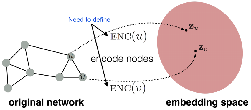
Learning Node embeddings:

Define an encoder (i.e., a mapping from nodes to embeddings).
Define a node similarity function (i.e., a measure of similarity in the original network).

Optimize the parameters of the encoder so that: Similarity (u, v) ≈ z^T_vz_u.

Two components:

Encoder: maps each node to a low dimensional vector. Enc(v) = z_v where v is node in the input graph and z_v is d-dimensional embedding.
Similarity function: specifies how the relationships in vector space map to the relationships in the original network – z^T_vz_uis a dot product between node embeddings.

“Shallow” encoding

The simplest encoding approach is when encoder is just an embedding-lookup.

Enc(v) = Zv where Z is a matrix with each column being a node embedding (what we learn) and v is an indicator vector with all zeroes except one in column indicating node v.

*Each node is assigned to a unique embedding vector*

Many methods for encoding: DeepWalk, node2vec, TransE. The methods are different in how they define node similarity (should two nodes have similar embeddings if they are connected or share neighbors or have similar “structural roles”?).

Random Walk approaches to node embeddings

Given a graph and a starting point, we select a neighbor of it at random, and move to this neighbor; then we select a neighbor of this point at random, and move to it, etc. The (random) sequence of points selected this way is a random walk on the graph.

Then z^T_vz_u ≈ probability that u and v co-occur on a random walk over the network.

Properties of random walks:

Expressivity: Flexible stochastic definition of node similarity that incorporates both local and higher-order neighbourhood information.
Efficiency: Do not need to consider all node pairs when training; only need to consider pairs that co-occur on random walks.

Algorithm:

Run short fixed-length random walks starting from each node on the graph using some strategy R.
For each node u collect N_R(u), the multiset (nodes can repeat) of nodes visited on random walks starting from u.

Optimize embeddings: given node u, predict its neighbours N_R(u)

$max_{z}\sum_{u \in V}^{}logP(N_R(u)|z_u) \rightarrow \Lambda =\sum_{u \in V} \sum_{v \in N_R(u)}-log(P(v|z_u))$

Intuition: Optimize embeddings to maximize likelihood of random walk co-occurrences.

Then parameterize it using softmax:

$\Lambda =\sum_{u \in V} \sum_{v \in N_R(u)}-log(\frac{exp(z_u^Tz_v)}{\sum_{n \in V}exp(z_u^Tz_n)})$

where first sum is sum over all nodes u, second sum is sum over nodes v seen on random walks starting from u and fraction (under log) is predicted probability of u and v co-occuring on random walk.

Optimizing random walk embeddings = Finding embeddings z_u that minimize Λ. Naive optimization is too expensive, use negative sampling to approximate.

Strategies for random walk itself:

Simplest idea: just run fixed-length, unbiased random walks starting from each node (i.e., DeepWalk from Perozzi et al., 2013). But such notion of similarity is too constrained.
More general: node2vec.

Node2vec: biased walks

Idea: use flexible, biased random walks that can trade off between local and global views of the network (Grover and Leskovec, 2016).

Two parameters:

Return parameter p: return back to the previous node
In-out parameter q: moving outwards (DFS) vs. inwards (BFS). Intuitively, q is the “ratio” of BFS vs. DFS

*Recap Breadth-first search and Depth-first search.*

Node2vec algorithm:

Compute random walk probabilities.
Simulate r random walks of length l starting from each node u.
Optimize the node2vec objective using Stochastic Gradient Descent.

How to use embeddings z_i of nodes:

Clustering/community detection: Cluster points z_i.
Node classification: Predict label f(z_i) of node i based on z_i.
Link prediction: Predict edge (i,j) based on f(z_i,z_j) with concatenation, avg, product, or the difference between the embeddings.

Random walk approaches are generally more efficient.

Translating embeddings for modeling multi-relational data

A knowledge graph is composed of facts/statements about inter-related entities. Nodes are referred to as entities, edges as relations. In Knowledge graphs (KGs), edges can be of many types!

Knowledge graphs may have missing relation. Intuition: we want a link prediction model that learns from local and global connectivity patterns in the KG, taking into account entities and relationships of different types at the same time.

Downstream task: relation predictions are performed by using the learned patterns to generalize observed relationships between an entity of interest and all the other entities.

In Translating Embeddings method (TransE), relationships between entities are represented as triplets h (head entity), l (relation), t (tail entity) => (ℎ, l, t).

Entities are first embedded in an entity space R^k and relations are represented as translations ℎ + l ≈ t if the given fact is true, else, ℎ + l ≠ t.

Embedding entire graphs

Sometimes we need to embed entire graphs to such tasks as classifying toxic vs. non-toxic molecules or identifying anomalous graphs.

Approach 1:

Run a standard graph embedding technique on the (sub)graph G. Then just sum (or average) the node embeddings in the (sub)graph G. (Duvenaud et al., 2016- classifying molecules based on their graph structure).

Approach 2:

Idea: Introduce a “virtual node” to represent the (sub)graph and run a standard graph embedding technique (proposed by Li et al., 2016 as a general technique for subgraph embedding).

Approach 3 – Anonymous Walk Embeddings:

States in anonymous walk correspond to the index of the first time we visited the node in a random walk.

*Number of anonymous walks grows exponentially with increasing length of a walk.*

Anonymous Walk Embeddings have 3 methods:

Represent the graph via the distribution over all the anonymous walks (enumerate all possible anonymous walks a_i of l steps, record their counts and translate it to probability distribution.
Create super-node that spans the (sub) graph and then embed that node (as complete counting of all anonymous walks in a large graph may be infeasible, sample to approximating the true distribution: generate independently a set of m random walks and calculate its corresponding empirical distribution of anonymous walks).
Embed anonymous walks (learn embedding z_i of every anonymous walk a_i. The embedding of a graph G is then sum/avg/concatenation of walk embeddings z_i).

Lecture 8 – Graph Neural Networks

Slides, Video

Recap that the goal of node embeddings it to map nodes so that similarity in the embedding space approximates similarity in the network. Last lecture was focused on “shallow” encoders, i.e. embedding lookups. This lecture will discuss deep methods based on graph neural networks:

Enc(v) = multiple layers of non-linear transformations of graph structure.

Modern deep learning toolbox is designed for simple sequences & grids. But networks are far more complex because they have arbitrary size and complex topological structure (i.e., no spatial locality like grids), no fixed node ordering or reference point and they often are dynamic and have multimodal features.

Naive approach of applying CNN to networks:

Join adjacency matrix and features.
Feed them into a deep neural net.

Issues with this idea: O(N) parameters; not applicable to graphs of different sizes; not invariant to node ordering.

Basics of Deep Learning for graphs

Setup: graph G with vertex set V, adjacency matrix A (assume binary), matrix of node features X (like user profile and images for social networks, gene expression profiles and gene functional information for biological networks; for case with no features it can be indicator vectors (one-hot encoding of a node) or vector of constant 1 [1, 1, …, 1]).

Idea: node’s neighborhood defines a computation graph -> generate node embeddings based on local network neighborhoods. Intuition behind the idea: nodes aggregate information from their neighbors using neural networks.

*Every node defines a computation graph based on its neighborhood*

Model can be of arbitrary depth:

Nodes have embeddings at each layer.
Layer-0 embedding of node x is its input feature, x_u.
Layer-K embedding gets information from nodes that are K hops away.

Different models vary in how they aggregate information across the layers (how neighbourhood aggregation is done).

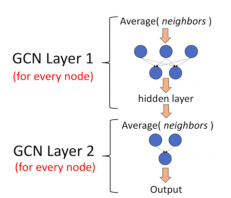
Basic approach is to average the information from neighbors and apply a neural network.

Initial 0-th layer embeddings are equal to node features: h_v⁰ = x_v. The next ones:

$h_v^k=\sigma(W_k \sum _ {u \in N(v)} \frac {h_v^{k-1}}{|N(v)}+B_kh_v^{k-1}), \forall k \in (1,...,K)$

where σ is non-linearity (e.g., ReLU), h_v^k-1 is previous layer embedding of v, sum (after W_k) is average v-th neghbour’s previous layer embeddings.

Embedding after K layers of neighborhood aggregation: z_v = h_v^K.

We can feed these embeddings into any loss function and run stochastic gradient descent to train the weight parameters. We can train in two ways:

Unsupervised manner: use only the graph structure.
- “Similar” nodes have similar embeddings.
- Unsupervised loss function can be anything from random walks (node2vec, DeepWalk, struc2vec), graph factorization, node proximity in the graph.
Supervised manner: directly train the model for a supervised task (e.g., node classification):

$\Lambda = \sum_{v \in V} y_v log(\sigma (z_v^T \theta))+(1-y_v)log(1-\sigma (z_v^T \theta))$

where z_v^T is encoder output (node embedding), y_v is node class label, θ is classigication weights.

Supervised training steps:

Define a neighborhood aggregation function
Define a loss function on the embeddings
Train on a set of nodes, i.e., a batch of compute graphs
Generate embeddings for nodes as needed

The same aggregation parameters are shared for all nodes:

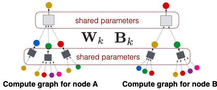
*The number of model parameters is sublinear in |V| and we can generalize to unseen nodes.*

The approach has inductive capability (generate embeddings for unseen nodes or graphs).

Graph Convolutional Networks and GraphSAGE

Can we do better than aggregating the neighbor messages by taking their (weighted) average (formula for h_v^k above)?

Variants

Mean: take a weighted average of neighbors:

$agg = \sum_{u \in N(v)} \frac {h_u^{k-1}}{|N(v)|}$

Pool: Transform neighbor vectors and apply symmetric vector function ( $\gamma$ is element-wise mean/max):

$agg = \gamma (\left \{ Qh_u^{k-1}, \forall u \in N(v) \right \})$

LSTM: Apply LSTM to reshuffled of neighbors:

$agg = LSTM(\left [ h_u^{k-1}, \forall u \in \pi (N(v)) \right ])$

Graph convolutional networks average neighborhood information and stack neural networks. Graph convolutional operator aggregates messages across neighborhoods, N(v).

a_vu = 1/|N(v)| is the weighting factor (importance) of node u’s message to node v. Thus, a_vu is defined explicitly based on the structural properties of the graph. All neighbors u ∈ N(v) are equally important to node v.

*Example of 2-layer GCN: The output of the first layer is the input of the second layer. Again, note that the neural network in GCN is simply a fully connected layer (*https://www.topbots.com/graph-convolutional-networks/)

GraphSAGE uses generalized neighborhood aggregation:

Graph Attention Networks

Idea: Compute embedding h_v^k of each node in the graph following an attention strategy:

Nodes attend over their neighborhoods’ message.
Implicitly specifying different weights to different nodes in a neighborhood.

Let a_vu be computed as a byproduct of an attention mechanism a. Let a compute attention coefficients e_vu across pairs of nodes u, v based on their messages: e_vu = a(W_kh_u^k-1,W_kh_v^k-1). e_vu indicates the importance of node u’s message to node v. Then normalize coefficients using the softmax function in order to be comparable across different neighborhoods:

$a_{vu} = \frac {exp(e_{vu})}{\sum _{k \in N(v)} exp(e_{vk})}$

$h_v^k= \sigma (\sum _{u \in N(v)} a_{vu}W_k h_u^{k-1})$

Form of attention mechanism a:

The approach is agnostic to the choice of a
- E.g., use a simple single-layer neural network.
- a can have parameters, which need to be estimates.
Parameters of a are trained jointly:
- Learn the parameters together with weight matrices (i.e., other parameter of the neural net) in an end-to-end fashion

Paper by Velickovic et al. introduced multi-head attention to stabilize the learning process of attention mechanism:

Attention operations in a given layer are independently replicated R times (each replica with different parameters). Outputs are aggregated (by concatenating or adding).
Key benefit: allows for (implicitly) specifying different importance values (a_vu) to different neighbors.
Computationally efficient: computation of attentional coefficients can be parallelized across all edges of the graph, aggregation may be parallelized across all nodes.
Storage efficient: sparse matrix operations do not require more than O(V+E) entries to be stored; fixed number of parameters, irrespective of graph size.
Trivially localized: only attends over local network neighborhoods.
Inductive capability: shared edge-wise mechanism, it does not depend on the global graph structure.

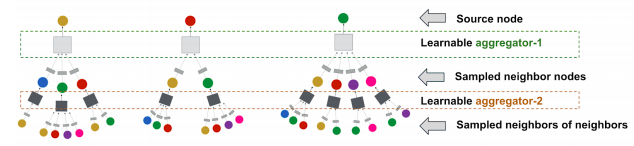
Example application: PinSage

Pinterest graph has 2B pins, 1B boards, 20B edges and it is dynamic. PinSage graph convolutional network:

Goal: generate embeddings for nodes (e.g., Pins/images) in a web-scale Pinterest graph containing billions of objects.
Key Idea: Borrow information from nearby nodes. E.g., bed rail Pin might look like a garden fence, but gates and beds are rarely adjacent in the graph.
Pin embeddings are essential to various tasks like recommendation of Pins, classification, clustering, ranking.
Challenges: large network and rich image/text features. How to scale the training as well as inference of node embeddings to graphs with billions of nodes and tens of billions of edges?
- To learn with resolution of 100 vs. 3B, they use harder and harder negative samples – include more and more hard negative samples for each epoch.

Key innovations:

On-the-fly graph convolutions:
- Sample the neighborhood around a node and dynamically construct a computation graph.
- Perform a localized graph convolution around a particular node.
- Does not need the entire graph during training.
Constructing convolutions via random walks:
- Performing convolutions on full neighborhoods is infeasible.
- Importance pooling to select the set of neighbors of a node to convolve over: define importance-based neighborhoods by simulating random walks and selecting the neighbors with the highest visit counts.
Efficient MapReduce inference:
- Bottom-up aggregation of node embeddings lends itself to MapReduce. Decompose each aggregation step across all nodes into three operations in MapReduce, i.e., map, join, and reduce.

*PinSage gives 150% improvement in hit rate and 60% improvement in MRR over the best baseline*

General tips working with GNN

Data preprocessing is important:
- Use renormalization tricks.
- Variance-scaled initialization.
- Network data whitening.
ADAM optimizer: naturally takes care of decaying the learning rate.
ReLU activation function often works really well.
No activation function at your output layer: easy mistake if you build layers with a shared function.
Include bias term in every layer.
GCN layer of size 64 or 128 is already plenty.

Lecture 9 – Graph Neural Networks: Hands-on Session

Video

Colab Notebook has everything to get hands on with PyTorch Geometric. Check it out!

Lecture 10 – Deep Generative Models for Graphs

Slides, Video

In precious lectures, we covered graph encoders where outputs are graph embeddings. This lecture covers the opposite aspect – graph decoders where outputs are graph structures.

Problem of Graph Generation

Why is it important to generate realistic graphs (or synthetic graph given a large real graph)?

Generation: gives insight into the graph formation process.
Anomaly detection: abnormal behavior, evolution.
Predictions: predicting future from the past.
Simulations of novel graph structures.
Graph completion: many graphs are partially observed.
“What if” scenarios.

Graph Generation tasks:

Realistic graph generation: generate graphs that are similar to a given set of graphs [Focus of this lecture].
Goal-directed graph generation: generate graphs that optimize given objectives/constraints (drug molecule generation/optimization). Examples: discover highly drug-like molecules, complete an existing molecule to optimize a desired property.

*Drug discovery: complete an existing molecule to optimize a desired property*

Why Graph Generation tasks are hard:

Large and variable output space (for n nodes we need to generate n*n values; graph size (nodes, edges) varies).
Non-unique representations (n-node graph can be represented in n! ways; hard to compute/optimize objective functions (e.g., reconstruction of an error)).
Complex dependencies: edge formation has long-range dependencies (existence of an edge may depend on the entire graph).

Graph generative models

Setup: we want to learn a generative model from a set of data points (i.e., graphs) {x_i}; p_DATA(x) is the data distribution, which is never known to us, but we have sampled x_i ~ p_DATA(x). p_MODEL(x,θ) is the model, parametrized by θ, that we use to approximate p_DATA(x).

Goal:

Make p_MODEL(x,θ) close to p_DATA(x) (Key Principle: Maximum Likelihood – find the model that is most likely to have generated the observed data x).
Make sure we can sample from a complex distribution p_MODEL(x,θ). The most common approach:
- Sample from a simple noise distribution z_i~ N(0,1).
- Transform the noise z_i via f(⋅): x_i= f(z_i; θ). Then x_i follows a complex distribution.

To design f(⋅) use Deep Neural Networks, and train it using the data we have.

This lecture is focused on auto-regressive models (predict future behavior based on past behavior). Recap autoregressive models: p_MODEL(x,θ) is used for both density estimation and sampling (from the probability density). Then apply chain rule: joint distribution is a product of conditional distributions:

$p_{model}(x; \theta)=\prod_{t=1}^{n} p_{model}(x_t | x_1,...,x_{t-1};\theta)$

In our case: x_t will be the t-th action (add node, add edge).

GraphRNN

[You et al., ICML 2018]

Idea: generating graphs via sequentially adding nodes and edges. Graph G with node ordering π can be uniquely mapped into a sequence of node and edge additions S^π.

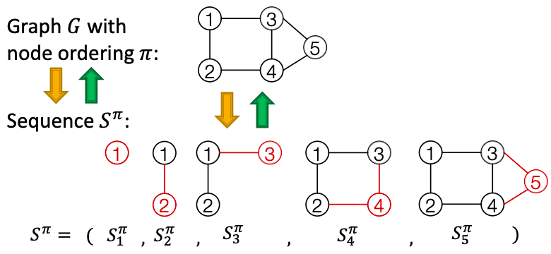
The sequence S^π has two levels:

Node-level: at each step, add a new node.
Edge-level: at each step, add a new edge/edges between existing nodes. For example, step 4 for picture above S^π₄ = (S^π_4,1, S^π_4,2, S^π₄₃₁: 0,1,1) means to connect 4&2, 4&3, but not 4&1).

Thus, S is a sequence of sequences: a graph + a node ordering. Node ordering is randomly selected.

We have transformed the graph generation problem into a sequence generation problem. Now we need to model two processes: generate a state for a new node (Node-level sequence) and generate edges for the new node based on its state (Edge-level sequence). We use RNN to model these processes.

GraphRNN has a node-level RNN and an edge-level RNN. Relationship between the two RNNs:

Node-level RNN generates the initial state for edge-level RNN.
Edge-level RNN generates edges for the new node, then updates node-level RNN state using generated results.

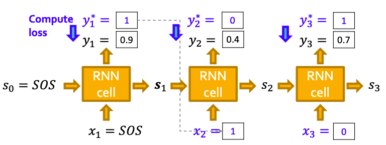
Setup: State of RNN after time s_t, input to RNN at time x_t, output of RNN at time y_t, parameter matrices W, U, V, non-linearity σ(⋅). s_t = σ(W⋅x_t+ U⋅ s_t-1 ), y_t = V⋅ s_t

To initialize s₀, x₁, use start/end of sequence token (SOS, EOS)- e.g., zero vector. To generate sequences we could let x_t+1 = y_t. but this model is deterministic. That’s why we use y_t = p_model(x_t|x₁, …, x_t-1; θ). Then x_t+1 is a sample from y_t: x_t+1~ y_t. In other words, each step of RNN outputs a probability vector; we then sample from the vector, and feed the sample to the next step.

During training process, we use Teacher Forcing principle depicted below: replace input and output by the real sequence.

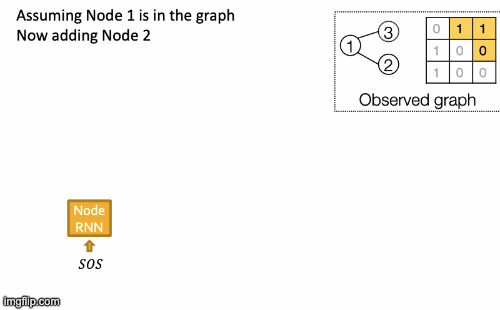
RNN steps:

Assume Node 1 is in the graph. Then add Node 2.
Edge RNN predicts how Node 2 connects to Node 1.
Edge RNN gets supervisions from ground truth.
New edges are used to update Node RNN.
Edge RNN predicts how Node 3 connects to Node 2.
Edge RNN gets supervisions from ground truth.
New edges are used to update Node RNN.
Node 4 doesn’t connect to any nodes, stop generation.
Backprop through time: All gradients are accumulated across time steps.
Replace ground truth by GraphRNN’s own predictions.

GraphRNN has an issue – tractability:

Any node can connect to any prior node.
Too many steps for edge generation:
- Need to generate a full adjacency matrix.
- Complex long edge dependencies.

Steps to generate graph below: Add node 1 – Add node 2 – Add node 3 – Connect 3 with 1 and 2 – Add node 4. But then Node 5 may connect to any/all previous nodes.

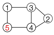
To limit this complexity, apply Breadth-First Search (BFS) node ordering. Steps with BFS: Add node 1 – Add node 2 – Connect 2 with 1 – Add node 3 – Connect 3 with 1 – Add node 4 – Connect 4 with 2 and 3. Since Node 4 doesn’t connect to Node 1, we know all Node 1’s neighbors have already been traversed. Therefore, Node 5 and the following nodes will never connect to node 1. We only need memory of 2 “steps” rather than n − 1 steps.

Benefits:

Reduce possible node orderings: from O(n!) to the number of distinct BFS orderings.
Reduce steps for edge generation (number of previous nodes to look at).

*BFS reduces the number of steps for edge generation*

When we want to define similarity metrics for graphs, the challenge is that there is no efficient Graph Isomorphism test that can be applied to any class of graphs. The solution is to use a visual similarity or graph statistics similarity.

Application: Drug Discovery

[You et al., NeurIPS 2018]

To learn a model that can generate valid and realistic molecules with high value of a given chemical property, one can use Goal-Directed Graph Generation which:

Optimize a given objective (High scores), e.g., drug-likeness (black box).
Obey underlying rules (Valid), e.g., chemical valency rules.
Are learned from examples (Realistic), e.g., imitating a molecule graph dataset.

Authors of paper present Graph Convolutional Policy Network that combines graph representation and RL. Graph Neural Network captures complex structural information, and enables validity check in each state transition (Valid), Reinforcement learning optimizes intermediate/final rewards (High scores) and adversarial training imitates examples in given datasets (Realistic).

*GCPN for generating graphs with high property scores*

*GCPN for editing given graph for higher property scores*

Open problems in graph generation

Generating graphs in other domains:
- 3D shapes, point clouds, scene graphs, etc.
Scale up to large graphs:
- Hierarchical action space, allowing high level action like adding a structure at a time.
Other applications: Anomaly detection.
- Use generative models to estimate probability of real graphs vs. fake graphs.

Lecture 11 – Link Analysis: PageRank

Slides, Video

The lecture covers analysis of the Web as a graph. Web pages are considered as nodes, hyperlinks are as edges. In the early days of the Web links were navigational. Today many links are transactional (used to navigate not from page to page, but to post, comment, like, buy, …).

The Web is directed graph since links direct from source to destination pages. For all nodes we can define IN-set (what other nodes can reach v?) and OUT-set (given node v, what nodes can v reach?).

Generally, there are two types of directed graphs:

Strongly connected: any node can reach any node via a directed path.
Directed Acyclic Graph (DAG) has no cycles: if u can reach v, then v cannot reach u.

Any directed graph (the Web) can be expressed in terms of these two types.

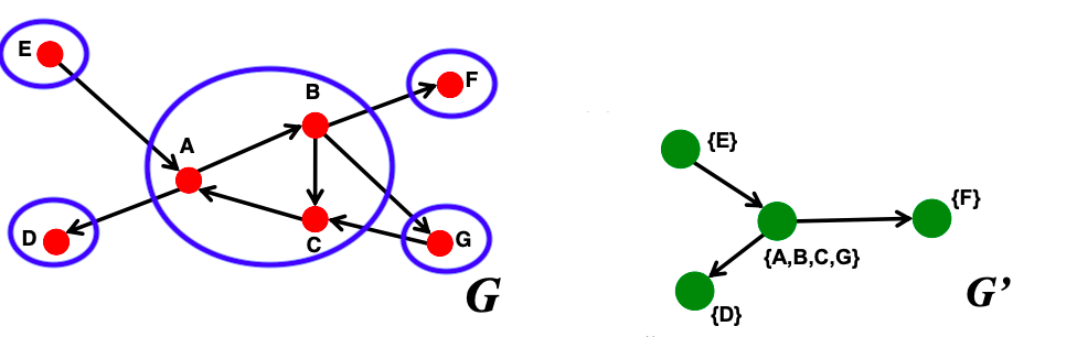
A Strongly Connected Component (SCC) is a set of nodes S so that every pair of nodes in S can reach each other and there is no larger set containing S with this property.

Every directed graph is a DAG on its SCCs:

SCCs partitions the nodes of G (that is, each node is in exactly one SCC).
If we build a graph G’ whose nodes are SCCs, and with an edge between nodes of G’ if there is an edge between corresponding SCCs in G, then G’ is a DAG.

*Strongly connected components of the graph G: {A,B,C,G}, {D}, {E}, {F}. G’ is a DAG*

Broder et al.: Altavista web crawl (Oct ’99): took a large snapshot of the Web (203 million URLS and 1.5 billion links) to understand how its SCCs “fit together” as a DAG.

Authors computed IN(v) and OUT(v) by starting at random nodes. The BFS either visits many nodes or very few as seen on the plot below:

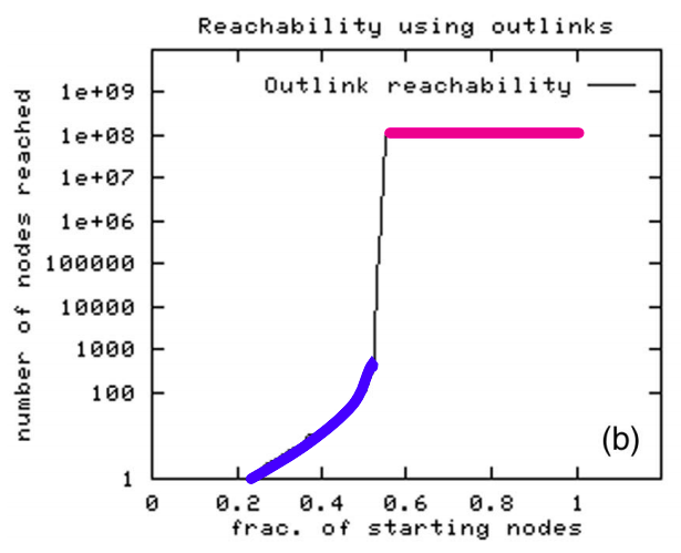
Based on IN and OUT of a random node v they found Out(v) ≈ 100 million (50% nodes), In(v) ≈ 100 million (50% nodes), largest SCC: 56 million (28% nodes). It shows that the web has so called “Bowtie” structure:

PageRank

There is a large diversity in the web-graph node connectivity -> all web pages are not equally “important”.

The main idea: page is more important if it has more links. They consider in-links as votes. A “vote” (link) from an important page is worth more:

Each link’s vote is proportional to the importance of its source page.
If page i with importance r_i has d_i out-links, each link gets r_i / d_i votes.
Page j’s own importance r_j is the sum of the votes on its in-links.

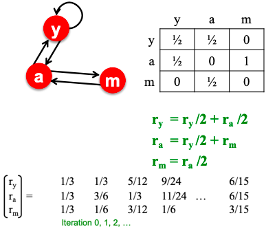
r_j = r_i /3 + r_k/4. Define a “rank” r_j for node j (d_i is out-degree of node i):

$r_j = \sum_{i\rightarrow j} \frac{r_i}{d_i}$

If we represent each node’s rank in this way, we get system of linear equations. To solve it, use matrix Formulation.

Let page j have d_j out-links. If node j is directed to i, then stochastic adjacency matrix M_ij = 1 / d_j . Its columns sum to 1. Define rank vector r – an entry per page: r_i is the importance score of page i, ∑r_i = 1. Then the flow equation is r = M ⋅ r.

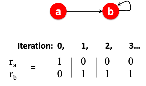
Random Walk Interpretation

Imagine a random web surfer. At any time t, surfer is on some page i. At time t + 1, the surfer follows an out-link from i uniformly at random. Ends up on some page j linked from i. Process repeats indefinitely. Then p(t) is a probability distribution over pages, it’s a vector whose i^th coordinate is the probability that the surfer is at page i at time t.

To identify where the surfer is at time t+1, follow a link uniformly at random p(t+1) = M ⋅ p(t). Suppose the random walk reaches a state p(t+1) = M ⋅ p(t) = p(t). Then p(t) is stationary distribution of a random walk. Our original rank vector r satisfies r = M ⋅ r. So, r is a stationary distribution for the random walk.

As flow equations is r = M ⋅ r, r is an eigenvector of the stochastic web matrix M. But Starting from any vector u, the limit M(M(…(M(Mu))) is the long-term distribution of the surfers. With math we derive that limiting distribution is the principal eigenvector of M – PageRank. Note: If r is the limit of M(M(…(M(Mu)), then r satisfies the equation r = M ⋅ r, so r is an eigenvector of M with eigenvalue 1. Knowing that, we can now efficiently solve for r with the Power iteration method.

Power iteration is a simple iterative scheme:

Initialize: r⁽⁰⁾ = [1/N,….,1/N]^T
Iterate: r^(t+1) = M · r^(t)
Stop when |r^(t+1) – r^(t)|₁ < ε (Note that |x|₁ = Σ|x_i| is the L1 norm, but we can use any other vector norm, e.g., Euclidean). About 50 iterations is sufficient to estimate the limiting solution.

How to solve PageRank

Given a web graph with n nodes, where the nodes are pages and edges are hyperlinks:

Assign each node an initial page rank.
Repeat until convergence (Σ |r^(t+1) – r^(t)|₁ < ε).

Calculate the page rank of each node (d_i …. out-degree of node i):

$r_j^{(t+1)} = \sum_{i\rightarrow j} \frac{r_i^{(t)}}{d_i}$

PageRank solution poses 3 questions: Does this converge? Does it converge to what we want? Are results reasonable?

PageRank has some problems:

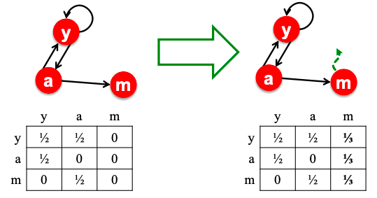
Some pages are dead ends (have no out-links, right part of web “bowtie”): such pages cause importance to “leak out”.
Spider traps (all out-links are within the group, left part of web “bowtie”): eventually spider traps absorb all importance.

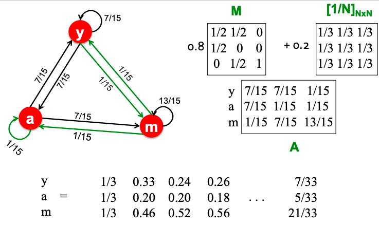
Solution for spider traps: at each time step, the random surfer has two options:

With probability β, follow a link at random.
With probability 1-β, jump to a random page.

Common values for β are in the range 0.8 to 0.9. Surfer will teleport out of spider trap within a few time steps.

Solution to Dead Ends: Teleports – follow random teleport links with total probability 1.0 from dead-ends (and adjust matrix accordingly)

Why are dead-ends and spider traps a problem and why do teleports solve the problem?

Spider-traps are not a problem, but with traps PageRank scores are not what we want.
- Solution: never get stuck in a spider trap by teleporting out of it in a finite number of steps.
Dead-ends are a problem: the matrix is not column stochastic so our initial assumptions are not met.
- Solution: make matrix column stochastic by always teleporting when there is nowhere else to go.

This leads to PageRank equation [Brin-Page, 98]:

$r_j = \sum_{i\rightarrow j} \beta \frac{r_i}{d_i}+(1- \beta) \frac{1}{N}$

This formulation assumes that M has no dead ends. We can either preprocess matrix M to remove all dead ends or explicitly follow random teleport links with probability 1.0 from dead-ends. (d_i … out-degree of node i).

The Google Matrix A becomes as:

$A = \beta M + (1 - \beta) \left [ \frac{1}{N} \right ]_{N\times N}$

[1/N]_NxN…N by N matrix where all entries are 1/N.

We have a recursive problem: r = A ⋅ r and the Power method still works.

Computing Pagerank

The key step is matrix-vector multiplication: r_new = A · r_old. Easy if we have enough main memory to hold each of them. With 1 bln pages, matrix A will have N² entries and 10¹⁸ is a large number.

But we can rearrange the PageRank equation

$r = \beta M\cdot r +\left [ \frac{1-\beta}{N} \right ]_N$

where [(1-β)/N]_N is a vector with all N entries (1-β)/N.

M is a sparse matrix (with no dead-ends):10 links per node, approx 10N entries. So in each iteration, we need to: compute r_new = β M · r_old and add a constant value (1-β)/N to each entry in r_new. Note if M contains dead-ends then ∑r_{j new} < 1 and we also have to renormalize r_new so that it sums to 1.

*Complete PageRank algorithm with input Graph G and parameter β*

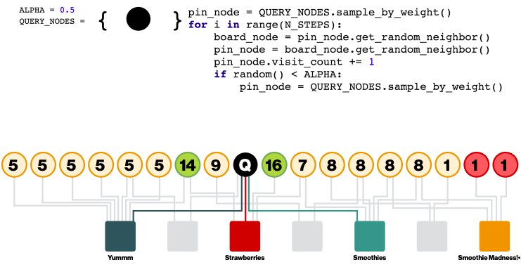
Random Walk with Restarts

Idea: every node has some importance; importance gets evenly split among all edges and pushed to the neighbors. Given a set of QUERY_NODES, we simulate a random walk:

Make a step to a random neighbor and record the visit (visit count).
With probability ALPHA, restart the walk at one of the QUERY_NODES.
The nodes with the highest visit count have highest proximity to the QUERY_NODES.

The benefits of this approach is that it considers: multiple connections, multiple paths, direct and indirect connections, degree of the node.

PS: Other lecture notes you can find here: 1, 3, 4.