Recently, I finished the Stanford course CS224W Machine Learning with Graphs. In the following series of blog posts, I share my notes which I took watching lectures. I hope it gives you a quick sneak peek overview of how ML applied for graphs. The rest of the blog posts you can find here: 2, 3, 4.

NB: I don’t have proofs and derivations of theorems here, check out original sources if you are interested.

Lecture 1 – Intro to graph theory
Lecture 2 – Properties of networks. Random Graphs
Recitation 1 – Introduction to snap.py
Lecture 3 – Motifs and Structural Roles in Networks
Lecture 4 – Community Structure in Networks
Lecture 5 – Spectral Clustering

Lecture 1 – Intro to graph theory

Slides, Video

The lecture gives an overview of basic terms and definitions used in graph theory. Why should you learn graphs? The impact! The impact of graphs application is proven for Social networking, Drug design, AI reasoning.

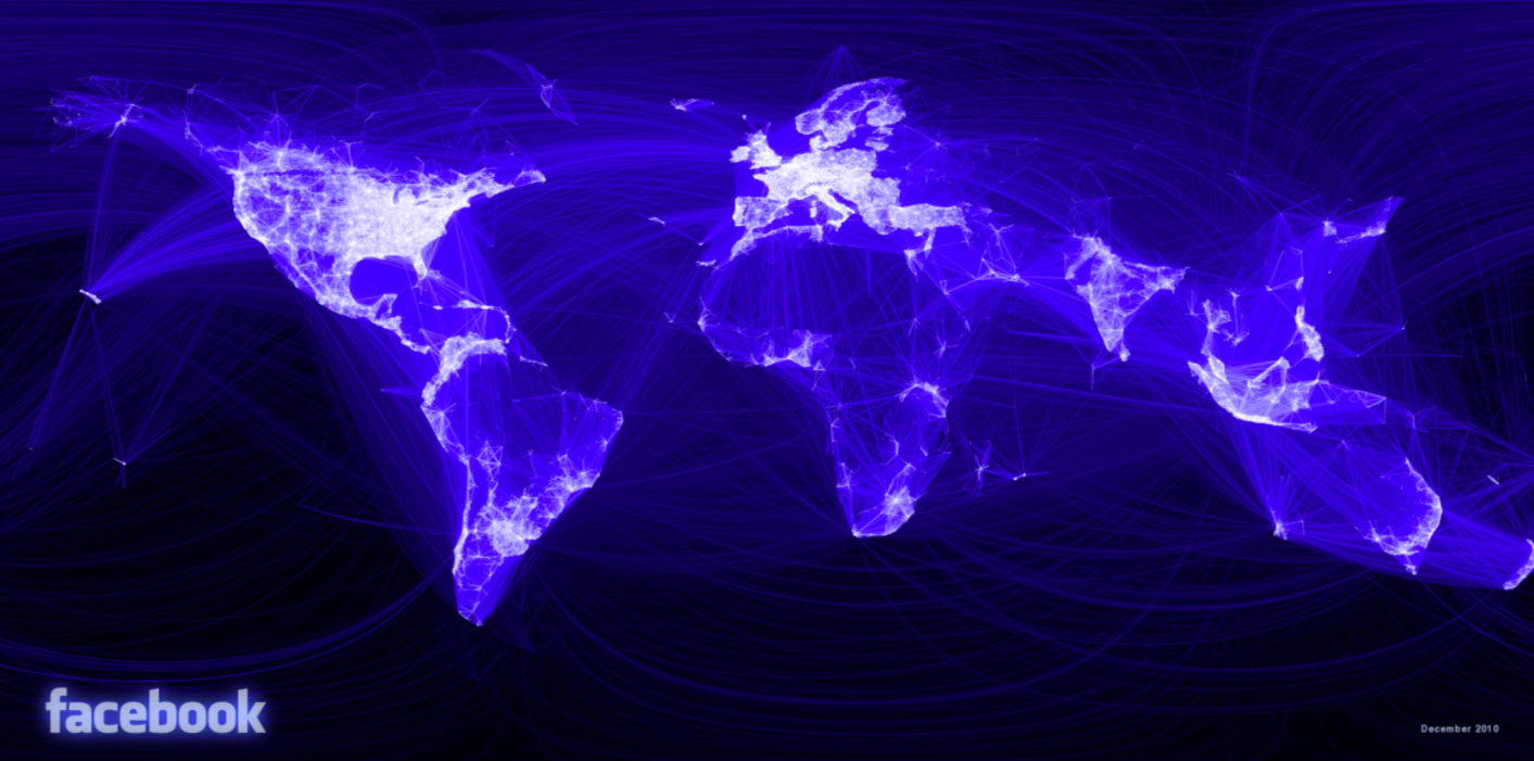
My favourite example of applications is the Facebook social graph which shows that all users have only 4-degrees of separation:

*[Backstrom-Boldi-Rosa-Ugander-Vigna, 2011]*

Another interesting example of application: predict side-effects of drugs (when patients take multiple drugs at the same time, what are the potential side effects? It represents a link prediction task).

What are the ways to analyze networks:

Node classification (Predict the type/color of a given node)
Link prediction (Predict whether two nodes are linked)
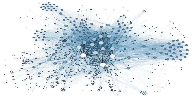
Identify densely linked clusters of nodes (Community detection)
Network similarity (Measure similarity of two nodes/networks)

Key definitions:

A network is a collection of objects (nodes) where some pairs of objects are connected by links (edges).
Types of networks: Directed vs. undirected, weighted vs. unweighted, connected vs. disconnected
Degree of node i is the number of edges adjacent to node i.
The maximum number of edges on N nodes (for undirected graph) is

$E_{max}=\frac{N(N-1)}{2}$

Complete graph is an undirected graph with the number of edges E = E_max, and its average degree is N-1.
Bipartite graph is a graph whose nodes can be divided into two disjoint sets U and V such that every link connects a node in U to one in V; that is, U and V are independent sets (restaurants-eaters for food delivery, riders-drivers for ride-hailing).
Ways for presenting a graph: visual, adjacency matrix, adjacency list.

Lecture 2 – Properties of networks. Random Graphs

Slides, Video

Metrics to measure network:

Degree distribution, P(k): Probability that a randomly chosen node has degree k.

N_k = # nodes with degree k.

Path length, h: a length of the sequence of nodes in which each node is linked to the next one (path can intersect itself).
Distance (shortest path, geodesic) between a pair of nodes is defined as the number of edges along the shortest path connecting the nodes. If the two nodes are not connected, the distance is usually defined as infinite (or zero).
Diameter: maximum (shortest path) distance between any pair of nodes in a graph.
Clustering coefficient, C_i: describes how connected are i’s neighbors to each other.

$C_{i}\in [0,1], C_{i}=\frac{2e_{i}}{k_{i}(k_{i}-1)}$

where e_i is the number of edges between neighbors of node i.

Average clustering coefficient:

$C=\frac{1}{N}\sum_{i}^{N}C_{i}$

Connected components, s: a subgraph in which each pair of nodes is connected with each other via a path (for real-life graphs, they usually calculate metrics for the largest connected components disregarding unconnected nodes).

Erdös-Renyi Random Graphs:

G_np: undirected graph on n nodes where each edge (u,v) appears i.i.d. with probability p.
Degree distribution of G_np is binomial.
Average path length: O(log n).
Average clustering coefficient: k / n.
Largest connected component: exists if k > 1.

Comparing metrics of random graph and real life graphs, real networks are not random. While G_np is wrong, it will turn out to be extremely useful!

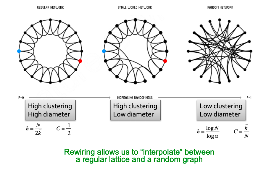
Real graphs have high clustering but diameter is also high. How can we have both in a model? Answer in Small-World Model [Watts-Strogatz ‘98].

Small-World Model introduces randomness (“shortcuts”): first, add/remove edges to create shortcuts to join remote parts of the lattice; then for each edge, with probability p, move the other endpoint to a random node.

*Difference between regular random and small world networks*

Kronecker graphs: a recursive model of network structure obtained by growing a sequence of graphs by iterating the Kronecker product over the initiator matrix. It may be illustrated in the following way:

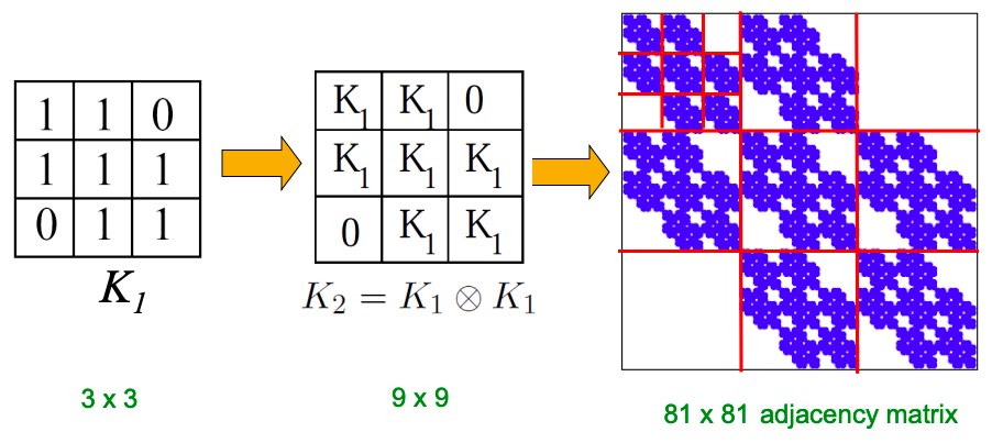
Random graphs are far away from real ones, but real and Kronecker networks are very close.

Recitation 1 – Introduction to snap.py

Slides

Stanford Network Analysis Platform (SNAP) is a general purpose, high-performance system for analysis and manipulation of large networks (http://snap.stanford.edu). SNAP software includes Snap.py for Python, SNAP C++ and SNAP datasets (over 70 network datasets can be found at https://snap.stanford.edu/data/).

Useful resources for plotting graph properties:

Gnuplot: http://www.gnuplot.info
Visualizing graphs with Graphviz: http://www.graphviz.org
Other options are in Matplotlib: http://www.matplotlib.org

I will not go into details here, better to get hands on right away with the original snappy tutorial at https://snap.stanford.edu/snappy/doc/tutorial/index-tut.html.

Lecture 3 – Motifs and Structural Roles in Networks

Slides, Video

Subnetworks, or subgraphs, are the building blocks of networks, they have the power to characterize and discriminate networks.

Network motifs are:

Recurring	found many times, i.e., with high frequency
Significant	Small induced subgraph: Induced subgraph of graph G is a graph, formed from a subset X of the vertices of graph G and all of the edges connecting pairs of vertices in subset X.
Patterns of interconnections	More frequent than expected. Subgraphs that occur in a real network much more often than in a random network have functional significance.

Motifs help us understand how networks work, predict operation and reaction of the network in a given situation.

Motifs can overlap each other in a network.

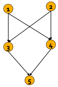
Examples of motifs:

Significance of motifs: Motifs are overrepresented in a network when compared to randomized networks. Significance is defined as:

$SP_{i}=Z_{i}/\sqrt{\sum_{j}^{}Z_{j}^{2}}\: \: and \, \, \; \! Z_{i}=(N_{i}^{real}-\bar{N_{i}^{rand}})/std(N_{i}^{rand})$

where N_i^real is # of subgraphs of type i in network G^real and N_i^real is # of subgraphs of type i in network G^rand.

Z_i captures statistical significance of motif i.
Generally, larger networks display higher Z-scores.
To calculate Z_i, one counts subgraphs i in G^real, then counts subgraphs i in G^rand with a configuration model which has the same #(nodes), #(edges) and #(degree distribution) as G^real.

Graphlets

Graphlets are connected non-isomorphic subgraphs (induced subgraphs of any frequency). Graphlets differ from network motifs, since they must be induced subgraphs, whereas motifs are partial subgraphs. An induced subgraph must contain all edges between its nodes that are present in the large network, while a partial subgraph may contain only some of these edges. Moreover, graphlets do not need to be over-represented in the data when compared with randomized networks, while motifs do.

Node-level subgraph metrics:

Graphlet degree vector counts #(graphlets) that a node touches.
Graphlet Degree Vector (GDV) counts #(graphlets) that a node touches.

Graphlet degree vector provides a measure of a node’s local network topology: comparing vectors of two nodes provides a highly constraining measure of local topological similarity between them.

Finding size-k motifs/graphlets requires solving two challenges:

Enumerating all size-k connected subgraphs
Counting # of occurrences of each subgraph type via graph isomorphisms test.

Just knowing if a certain subgraph exists in a graph is a hard computational problem!

Subgraph isomorphism is NP-complete.
Computation time grows exponentially as the size of the motif/graphlet increases.
Feasible motif size is usually small (3 to 8).

Algorithms for counting subgaphs:

Exact subgraph enumeration (ESU) [Wernicke 2006] (explained in the lecture, I will not cover it here).
Kavosh [Kashani et al. 2009].
Subgraph sampling [Kashtan et al. 2004].

Structural roles in networks

Role is a collection of nodes which have similar positions in a network

Roles are based on the similarity of ties between subsets of nodes.
In contrast to groups/communities, nodes with the same role need not be in direct, or even indirect interaction with each other.
Examples: Roles of species in ecosystems, roles of individuals in companies.
Structural equivalence: Nodes are structurally equivalent if they have the same relationships to all other nodes.

*Nodes 3 and 4 are structurally equivalent*

Examples when we need roles in networks:

Role query: identify individuals with similar behavior to a known target.
Role outliers: identify individuals with unusual behavior.
Role dynamics: identify unusual changes in behavior.

Structural role discovery method RoIX:

Input is adjacency matrix.
Turn network connectivity into structural features with Recursive feature Extraction [Henderson, et al. 2011a]. Main idea is to aggregate features of a node (degree, mean weight, # of edges in egonet, mean clustering coefficient of neighbors, etc) and use them to generate new recursive features (e.g., mean value of “unweighted degree” feature between all neighbors of a node). Recursive features show what kinds of nodes the node itself is connected to.
Cluster nodes based on extracted features. RolX uses non negative matrix factorization for clustering, MDL for model selection, and KL divergence to measure likelihood.

Lecture 4 – Community Structure in Networks

Slides, Video

The lecture shows methods for community detection problems (nodes clustering).

Background example from Granovetter work, 1960s: people often find out about new jobs through acquaintances rather than close friends. This is surprising: one would expect your friends to help you out more than casual acquaintances.

Why is it that acquaintances are most helpful?

Long-range edges (socially weak, spanning different parts of the network) allow you to gather information from different parts of the network and get a job.
Structurally embedded edges (socially strong) are heavily redundant in terms of information access.

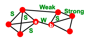
*Visualisation of strong and weak relations in a network*

From this observation we find one type of structural role – Triadic Closure: if two people in a network have a friend in common, then there is an increased likelihood they will become friends themselves.

Triadic closure has high clustering coefficient. Reasons: if A and B have a friend C in common, then:

A is more likely to meet B (since they both spend time with C).
A and B trust each other (since they have a friend in common).
C has incentive to bring A and B together (since it is hard for C to maintain two disjoint relationships).

Granovetter’s theory suggests that networks are composed of tightly connected sets of nodes and leads to the following conceptual picture of networks:

Network communities

Network communities are sets of nodes with lots of internal connections and few external ones (to the rest of the network).

Modularity is a measure of how well a network is partitioned into communities: the fraction of the edges that fall within the given groups minus the expected fraction if edges were distributed at random.

Given a partitioning of the network into groups disjoint s:

$s\in S: \enspace Q\propto \sum_{s\in S}^{}[(number \; of \; edges \; within \; group \; s)-(expected \; number \; of \; edges \; within \; group \; s)]$

Modularity values take range [−1,1]. It is positive if the number of edges within groups exceeds the expected number. Values greater than 0.3-0.7 means significant community structure.

To define the expected number of edges, we need a Null model. After derivations (can be found in slides), modularity is defined as:

$Q(G, S)=\frac{1}{2m}\sum_{s \in S}^{}\sum_{i \in s}^{}\sum_{j \in s}^{}(A_{ij}-\frac{k_{i}k_{j}}{2m})$

A_ij represents the edge weight between nodes i and j;
k_i and kj are the sum of the weights of the edges attached to nodes i and j;
2m is the sum of all the edges weights in the graph.

Louvian algorithm

Louvian algorithm is a greedy algorithm for community detection with O(n log(n)) run time.

Supports weighted graphs.
Provides hierarchical communities.
Widely utilized to study large networks because it is fast, has rapid convergence and high modularity output (i.e., “better communities”).

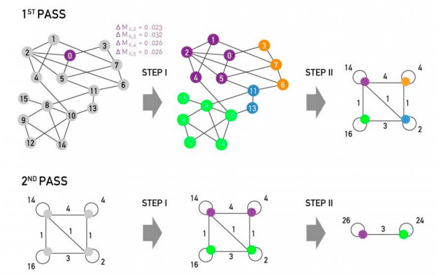
Each pass of Louvain algorithm is made of 2 phases:

Phase 1 – Partitioning:

Modularity is optimized by allowing only local changes to node-communities memberships;
For each node i, compute the modularity delta (∆Q) when putting node i into the community of some neighbor j;
Move i to a community of node j that yields the largest gain in ∆Q.

Phase 2 – Restructuring:

identified communities are aggregated into super-nodes to build a new network;
communities obtained in the first phase are contracted into super-nodes, and the network is created accordingly: super-nodes are connected if there is at least one edge between the nodes of the corresponding communities;
the weight of the edge between the two supernodes is the sum of the weights from all edges between their corresponding communities;
goto Phase 1 to run it on the super-node network.

The passes are repeated iteratively until no increase of modularity is possible.

Detecting overlapping communities: BigCLAM

BigCLAM is a model-based community detection algorithm that can detect densely overlapping, hierarchically nested as well as non-overlapping communities in massive networks (more details and all proofs are in Yang, Leskovec “Overlapping Community Detection at Scale: A Nonnegative Matrix Factorization Approach”, 2013).

In BigCLAM communities arise due to shared community affiliations of nodes. It explicitly models the affiliation strength of each node to each community. Model assigns each node-community pair a nonnegative latent factor which represents the degree of membership of a node to the community. It then models the probability of an edge between a pair of nodes in the network as a function of the shared community affiliations.

Step 1: Define a generative model for graphs that is based on node community affiliations – Community Affiliation Graph Model (AGM). Model parameters are Nodes V, Communities C, Memberships M. Each community c has a single probability p_c.

Step 2: Given graph G, make the assumption that G was generated by AGM. Find the best AGM that could have generated G. This way we discover communities.

Lecture 5 – Spectral Clustering

Slides, Video

NB: these notes skip lots of mathematical proofs, all derivations can be found in slides themselves.

Three basic stages of spectral clustering:

Pre-processing: construct a matrix representation of the graph.
Decomposition: compute eigenvalues and eigenvectors of the matrix; map each point to a lower-dimensional representation based on one or more eigenvectors.
Grouping: assign points to two or more clusters, based on the new representation.

Lecture covers them one by one starting with graph partitioning.

Graph partitioning

Bi-partitioning task is a division of vertices into two disjoint groups A and B. Good partitioning will maximize the number of within-group connections and minimize the number of between-group connections. To achieve this, define edge cut: a set of edges with one endpoint in each group:

$Cut(A,B)=\sum_{i \in A, j \in B}^{}w_{ij}$

Graph cut criterion:

Minimum-cut: minimize weight of connections between groups. Problems: it only considers external cluster connections and does not consider internal cluster connectivity.
Conductance: connectivity between groups relative to the density of each group. It produces more balanced partitions, but computing the best conductance cut is NP-hard.

Conductance φ(A,B) = cut(A, B) / min(total weighted degree of the nodes in A or in B)

To efficiently find good partitioning, they use Spectral Graph Theory.

Spectral Graph Theory analyze the “spectrum” of matrix representing G: Eigenvectors x⁽ⁱ⁾ of a graph, ordered by the magnitude (strength) of their corresponding eigenvalues λ_i.

Λ = {λ₁,λ₂,…,λ_n}, λ₁≤ λ₂≤ …≤ λ_n (λ_i are sorted in ascending (not descending) order).

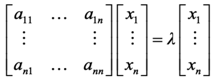
If A is adjacency matrix of undirected G (a_ij=1 if (i,j) is an edge, else 0), then Ax = λx.

What is the meaning of Ax? It is a sum of labels x_j of neighbors of i. It is better seen if represented in the form as below:

Examples of eigenvalues for different graphs:

For d-regular graph (where all nodes have degree d) if try x=(1,1,1,…1):

Ax = (d,d,..,d) = λx -> λ = d. This d is the largest eigenvalue of d-regular graph (proof is in slides).

An N x N matrix can have up to n eigenpairs.

Matrix Representation:

Adjacency matrix (A): A = [a_ij], a_ij = 1 if edge exists between node i and j (0-s on diagonal). It is a symmetric matrix, has n real eigenvalues; eigenvectors are real-valued and orthogonal.
Degree matrix (D): D=[d_ij],dijis a degree of node i.
Laplacian matrix (L): L = D-A. Trivial eigenpair is with x=(1,…,1) -> Lx = 0 and so λ = λ₁ = 0.

So far, we found λ and λ₁. From theorems, they derive

$\lambda _{2}=min \frac {\sum_{(i,j) \in E} (x_{i}-x_{j})^{2}}{\sum_{i}x_{i}^{2}}$

(all labelings of node i so that sum(x_i) = 0, meaning to assign values x_i to nodes i such that few edges cross 0 (x_i and x_j to subtract each other as shown on the picture below).

From theorems and profs, we go to the Cheeger inequality:

$\frac {\beta ^{2}}{2k_{max}}\leqslant \lambda _{2} \leqslant 2 \beta$

where k_max is the maximum node degree in the graph and β is conductance of the cut (A, B).

β = (# edges from A to B) / |A|. This is the approximation guarantee of the spectral clustering: spectral finds a cut that has at most twice the conductance as the optimal one of conductance β.

To summarize 3 steps of spectral clustering:

Pre-processing: build Laplacian matrix L of the graph.
Decomposition: find eigenvalues λ and eigenvectors x of the matrix L and map vertices to corresponding components of x₂.
Grouping: sort components of reduced 1-dimensional vector and identify clusters by splitting the sorted vector in two.

How to choose a splitting point?

Naïve approaches: split at 0 or median value.
More expensive approaches: attempt to minimize normalized cut in 1-dimension (sweep over ordering of nodes induced by the eigenvector).

K-way spectral clustering:

Recursive bi-partitioning [Hagen et al., ’92] is the method of recursively applying bi-partitioning algorithm in a hierarchical divisive manner. It has disadvantages: inefficient and unstable.

More preferred way:

Cluster multiple eigenvectors [Shi-Malik, ’00]: build a reduced space from multiple eigenvectors. Each node is now represented by k numbers; then we cluster (apply k-means) the nodes based on their k-dimensional representation.

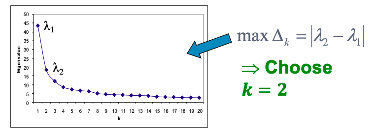
To select k, use eigengap: the difference between two consecutive eigenvalues (the most stable clustering is generally given by the value k that maximizes eigengap).

*K-way spectral clustering: choose k=2 as it has the highest eigengap.*

Motif-based spectral clustering

Different motifs will give different modular structures. Spectral clustering for nodes generalizes for motifs as well.

Similarly to edge cuts, volume and conductance, for motifs:

vol_M(S) = #(motif endpoints in S), φ(S) = #(motifs cut) / vol_M(S).

Motif Spectral Clustering works as follows:

Input: Graph G and motif M.
Using G form a new weighted graph W^(M).
Apply spectral clustering on W^(M).
Output the clusters.

Resulting clusters will obtain near optimal motif conductance.

The same 3 steps as before:

Preprocessing: given motif M. Form weighted graph W^(M).

W_ij^(M)=# times edge (i,j) participates in the motif M.

Apply spectral clustering: Compute Fiedler vector x associated with λ₂ of the Laplacian of L^(M).

L^(M) = D^(M) – W^(M) where degree matrix D_ij^(M) = sum(W_ij^(M)). Compute L^(M)x = λ₂x. Use x to identify communities.

Sort nodes by their values in x: x₁, x₂, …x_n. Let S_r = {x₁, x₂, …x_n} and compute the motif conductance of each S_r.

At the end of the lecture, there are two examples of how motif-based clustering is used for food webs and gene regulatory networks.

There exist other methods for clustering:

METIS: heuristic but works really well in practice.
Graclus: based on kernel k-means.
Louvain: based on Modularity optimization.
Clique percolation method: for finding overlapping clusters.

PS: Other lecture notes you can find here: 2, 3, 4.

Month: December 2020

Machine Learning with Graphs: lecture notes, part 1/4

Lecture 1 – Intro to graph theory

Lecture 2 – Properties of networks. Random Graphs

Erdös-Renyi Random Graphs:

Recitation 1 – Introduction to snap.py

Lecture 3 – Motifs and Structural Roles in Networks

Graphlets

Lecture 4 – Community Structure in Networks

Network communities

Louvian algorithm

Detecting overlapping communities: BigCLAM

Lecture 5 – Spectral Clustering

Graph partitioning

K-way spectral clustering:

Motif-based spectral clustering