Some time ago, I finished the Stanford course CS224W Machine Learning with Graphs. This is the last Part 4 of blog posts series where I share my notes from watching lectures. The rest you can find here: 1, 2, 3.
- Lecture 17 – Reasoning over Knowledge Graphs
- Lecture 18 – Limitations of Graph Neural Networks
- Lecture 19 – Applications of Graph Neural Networks
Lecture 17 – Reasoning over Knowledge Graphs
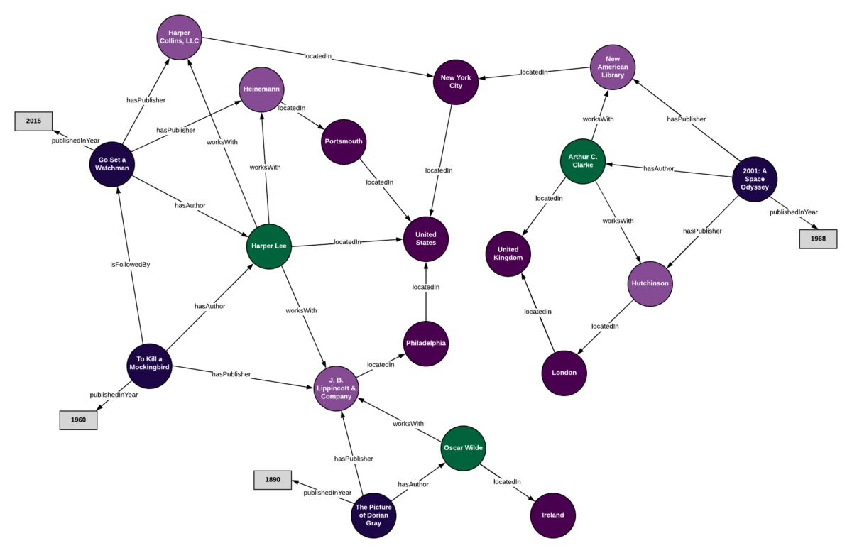
Knowledge graphs are graphs which capture entities, types, and relationships. Nodes in these graphs are entities that are labeled with their types and edges between two nodes capture relationships between entities.
Examples are bibliographical network (node types are paper, title, author, conference, year; relation types are pubWhere, pubYear, hasTitle, hasAuthor, cite), social network (node types are account, song, post, food, channel; relation types are friend, like, cook, watch, listen).
Knowledge graphs in practice:
- Google Knowledge Graph.
- Amazon Product Graph.
- Facebook Graph API.
- IBM Watson.
- Microsoft Satori.
- Project Hanover/Literome.
- LinkedIn Knowledge Graph.
- Yandex Object Answer.
Knowledge graphs (KG) are applied in different areas, among others are serving information and question answering and conversation agents.
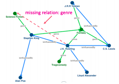
There exists several publicly available KGs (FreeBase, Wikidata, Dbpedia, YAGO, NELL, etc). They are massive (having millions of nodes and edges), but incomplete (many true edges are missing).
Given a massive KG, enumerating all the possible facts is intractable. Can we predict plausible BUT missing links?
Example: Freebase
- ~50 million entities.
- ~38K relation types.
- ~3 billion facts/triples.
- Full version is incomplete, e.g. 93.8% of persons from Freebase have no place of birth and 78.5% have no nationality.
- FB15k/FB15k-237 are complete subsets of Freebase, used by researchers to learn KG models.
- FB15k has 15K entities, 1.3K relations, 592K edges
- FB15k-237 has 14.5K entities, 237 relations, 310K edges
KG completion
We look into methods to understand how given an enormous KG we can complete the KG / predict missing relations.
Key idea of KG representation:
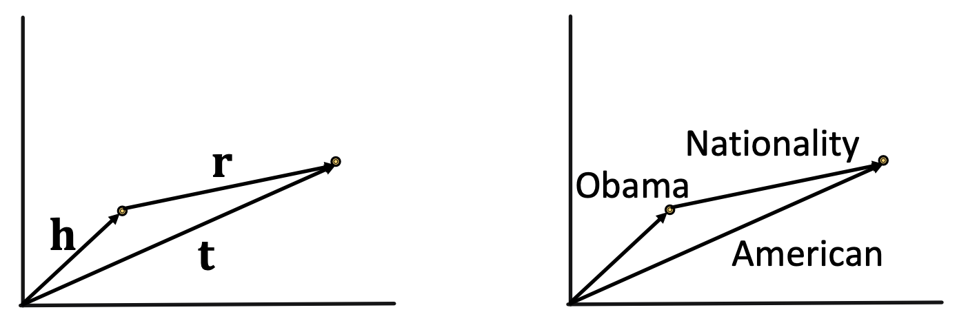
- Edges in KG are represented as triples (ℎ, r ,t) where head (ℎ) has relation (r) with tail (t).
- Model entities and relations in the embedding/vector space ℝd.
- Given a true triple (ℎ, r ,t), the goal is that the embedding of (ℎ, r) should be close to the embedding of t.
How to embed ℎ, r ? How to define closeness? Answer in TransE algorithm.
Translation Intuition: For a triple (ℎ, r ,t), ℎ, r ,t ∈ ℝd , h + r = t (embedding vectors will appear in boldface). Score function: fr(ℎ,t) = ||ℎ + r − t||
TransE training maximizes margin loss ℒ = Σfor (ℎ, r ,t)∈G, (ℎ, r ,t’)∉G [γ + fr(ℎ,t) − fr(ℎ,t’)]+ where γ is the margin, i.e., the smallest distance tolerated by the model between a valid triple (fr(ℎ,t)) and a corrupted one (fr(ℎ,t’) ).

Relation types in TransE
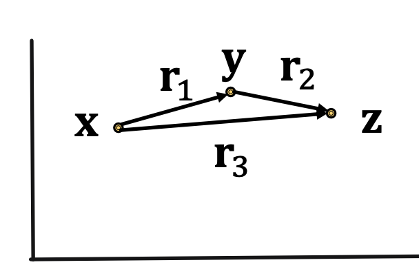
- Composition relations: r1 (x, y) ∧ r2 (y, z) ⇒ r3 (x,z) ∀ x, y, z (Example: My mother’s husband is my father). It satisfies TransE: r3 = r1 + r2 (look how it looks on 2D space below)
- Symmetric Relations: r (ℎ, t) ⇒ r (t, h) ∀ h, t (Example: Family, Roommate). It doesn’t satisfy TransE. If we want TransE to handle symmetric relations r, for all ℎ,t that satisfy r (ℎ, t), r (t, h) is also True, which means ‖ ℎ + r − t ‖ = 0 and ‖ t + r − ℎ ‖ = 0. Then r = 0 and ℎ = t, however ℎ and t are two different entities and should be mapped to different locations.
- 1-to-N, N-to-1, N-to-N relations: (ℎ, r ,t1) and (ℎ, r ,t2) both exist in the knowledge graph, e.g., r is “StudentsOf”. It doesn’t satisfy TransE. With TransE, t1 and t2 will map to the same vector, although they are different entities.

TransR
TransR algorithm models entities as vectors in the entity space ℝd and model each relation as vector r in relation space ℝk with Mr ∈ ℝk x d as the projection matrix.

Relation types in TransR
- Composition Relations: TransR doesn’t satisfy – Each relation has different space. It is not naturally compositional for multiple relations.
- Symmetric Relations: For TransR, we can map ℎ and t to the same location on the space of relation r.
- 1-to-N, N-to-1, N-to-N relations: We can learn Mr so that t⊥ = Mrt1 = Mrt2, note that t1 does not need to be equal to t2.

Types of queries on KG
- One-hop queries: Where did Hinton graduate?
- Path Queries: Where did Turing Award winners graduate?
- Conjunctive Queries: Where did Canadians with Turing Award graduate?
- EPFO (Existential Positive First-order): Queries Where did Canadians with Turing Award or Nobel graduate?
One-hop Queries
We can formulate one-hop queries as answering link prediction problems.
Link prediction: Is link (ℎ, r, t) True? -> One-hop query: Is t an answer to query (ℎ, r)?
We can generalize one-hop queries to path queries by adding more relations on the path.
Path Queries
Path queries can be represented by q = (va, r1, … , rn) where va is a constant node, answers are denoted by ||q||.
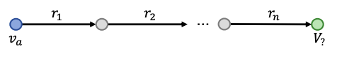
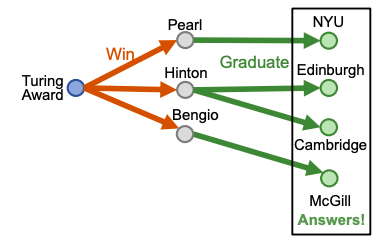
For example ““Where did Turing Award winners graduate?”, va is “Turing Award”, (r1, r2) is (“win”, “graduate”).
To answer path query, traverse KG: start from the anchor node “Turing Award” and traverse the KG by the relation “Win”, we reach entities {“Pearl”, “Hinton”, “Bengio”}. Then start from nodes {“Pearl”, “Hinton”, “Bengio”} and traverse the KG by the relation “Graduate”, we reach entities {“NYU”, “Edinburgh”, “Cambridge”, “McGill”}. These are the answers to the query.
How can we traverse if KG is incomplete? Can we first do link prediction and then traverse the completed (probabilistic) KG? The answer is no. The completed KG is a dense graph. Time complexity of traversing a dense KG with |V| entities to answer (va, r1, … , rn) of length n is O(|V|n).
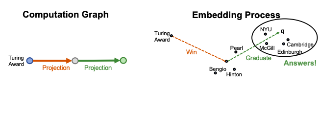
Another approach is to traverse KG in vector space. Key idea is to embed queries (generalize TransE to multi-hop reasoning). For v being an answer to q, do a nearest neighbor search for all v based on fq(v) = ||q − v||, time complexity is O(V).
Conjunctive Queries
We can answer more complex queries than path queries: we can start from multiple anchor nodes.
For example “Where did Canadian citizens with Turing Award graduate?”, start from the first anchor node “Turing Award”, and traverse by relation “Win”, we reach {“Pearl”, “Hinton”, “Bengio”}. Then start from the second anchor node “Canada”, and traverse by relation “citizen”, we reach { “Hinton”, “Bengio”, “Bieber”, “Trudeau”}. Then, we take the intersection of the two sets and achieve {‘Hinton’, ‘Bengio’}. After we do another traverse and arrive at the answers.

Again, another approach is to traverse KG in vector space. But how do we take the intersection of several vectors in the embedding space?
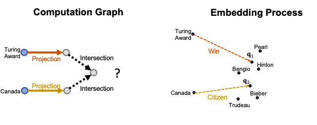
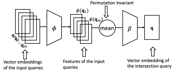
To do that, design a neural intersection operator ℐ:
- Input: current query embeddings q1, …, qm.
- Output: intersection query embedding q.
- ℐ should be permutation invariant: ℐ (q1, …, qm) = ℐ(qp(1), …, qp(m)), [p(1) , … , p(m) ] is any permutation of [1, … , m].

Training is the following: Given an entity embedding v and a query embedding q, the distance is fq(v) = ||q − v||. Trainable parameters are: entity embeddings d |V|, relation embeddings d |R|, intersection operator ϕ, β.
The whole process:
- Training:
- Sample a query q, answer v, negative sample v′.
- Embed the query q.
- Calculate the distance fq(v) and fq(v’).
- Optimize the loss ℒ.
- Query evaluation:
- Given a test query q, embed the query q.
- For all v in KG, calculate fq(v).
- Sort the distance and rank all v.
Taking the intersection between two vectors is an operation that does not follow intuition. When we traverse the KG to achieve the answers, each step produces a set of reachable entities. How can we better model these sets? Can we define a more expressive geometry to embed the queries? Yes, with Box Embeddings.
Query2Box: Reasoning with Box Embeddings
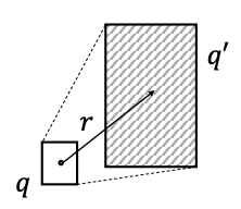
The idea is to embed queries with hyper-rectangles (boxes): q = (Center (q), Offset (q)).
Taking intersection between two vectors is an operation that does not follow intuition. But intersection of boxes is well-defined. Boxes are a powerful abstraction, as we can project the center and control the offset to model the set of entities enclosed in the box.
Parameters are similar to those before: entity embeddings d |V| (entities are seen as zero-volume boxes), relation embeddings 2d |R| (augment each relation with an offset), intersection operator ϕ, β (inputs are boxes and output is a box).
Also, now we have Geometric Projection Operator P: Box × Relation → Box: Cen (q’) = Cen (q) + Cen (r), Off (q’) = Off (q) + Off (r).
Another operator is Geometric Intersection Operator ℐ: Box × ⋯× Box → Box. The new center is a weighted average; the new offset shrinks.
Cen (qinter) = Σ wi ⊙ Cen (qi), Off (qinter) = min (Off (q1), …, Off (qn)) ⊙ σ (Deepsets (q1, …, qn)) where ⊙ is dimension-wise product, min function guarantees shrinking and sigmoid function σ squashes output in (0,1).


Entity-to-Box Distance: Given a query box q and entity vector v, dbox (q,v) = dout (q,v) + α din (q,v) where 0 < α < 1.
During training, Query2box minimises loss ℒ = − log σ (γ – dbox(q,v)) – log σ (γ – dbox(q,v’i) – γ)
Query2box can handle different relation patterns:
- Composition relations: r1 (x, y) ∧ r2 (y, z) ⇒ r3 (x,z) ∀ x, y, z (Example: My mother’s husband is my father). It satisfies Query2box: if y is in the box of (x, r1) and z is in the box of (y, r2), it is guaranteed that z is in the box of (x, r1 + r2).

- Symmetric Relations: r (ℎ, t) ⇒ r (t, h) ∀ h, t (Example: Family, Roommate). For symmetric relations r, we could assign Cen (r) = 0. In this case, as long as t is in the box of (ℎ, r), it is guaranteed that ℎ is in the box of (t, r). So we have r (ℎ, t) ⇒ r (t, h).
- 1-to-N, N-to-1, N-to-N relations: (ℎ, r ,t1) and (ℎ, r ,t2) both exist in the knowledge graph, e.g., r is “StudentsOf”. Box Embedding can handle since t1 and t2 will be mapped to different locations in the box of (ℎ, r).
EPFO queries
Can we embed even more complex queries? Conjunctive queries + disjunction is called Existential Positive First-order (EPFO) queries. E.g., “Where did Canadians with Turing Award or Nobel graduate?” Yes, we also can design a disjunction operator and embed EPFO queries in low-dimensional vector space.For details, they suggest to check the paper, but the link is not working (during the video they skipped this part, googling also didn’t help to find what exactly they meant…).
Lecture 18 – Limitations of Graph Neural Networks
Recap Graph Neural Networks: key idea is to generate node embeddings based on local network neighborhoods using neural networks. Many model variants have been proposed with different choices of neural networks (mean aggregation + Linear ReLu in GCN (Kipf & Welling ICLR’2017), max aggregation and MLP in GraphSAGE (Hamilton et al. NeurIPS’2017)).
Graph Neural Networks have achieved state-of the-art performance on:
- Node classification [Kipf+ ICLR’2017].
- Graph Classification [Ying+ NeurIPS’2018].
- Link Prediction [Zhang+ NeurIPS’2018].
But GNN are not perfect:
- Some simple graph structures cannot be distinguished by conventional GNNs.
- GNNs are not robust to noise in graph data (Node feature perturbation, edge addition/deletion).
Limitations of conventional GNNs in capturing graph structure
Given two different graphs, can GNNs map them into different graph representations? Essentially, it is a graph isomorphism test problem. No polynomial algorithms exist for the general case. Thus, GNNs may not perfectly distinguish any graphs.
To answer, how well can GNNs perform the graph isomorphism test, need to rethink the mechanism of how GNNs capture graph structure.
GNNs use different computational graphs to distinguish different graphs as shown on picture below:

Recall injectivity: the function is injective if it maps different elements into different outputs. Thus, entire neighbor aggregation is injective if every step of neighbor aggregation is injective.
Neighbor aggregation is essentially a function over multi-set (set with repeating elements) over multi-set (set with repeating elements). Now let’s characterize the discriminative power of GNNs by that of multi-set functions.
- GCN: as GCN uses mean pooling, it will fail to distinguish proportionally equivalent multi-sets (it is not injective).

- GraphSAGE: as it uses MLP and max pooling, it will even fail to distinguish multi-set with the same distinct elements (it is not injective).
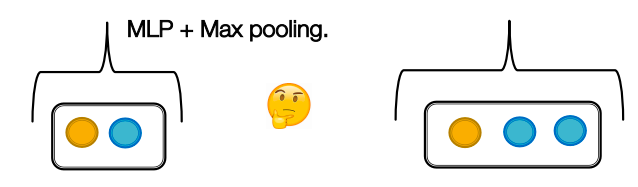
How can we design injective multi-set function using neural networks?
For that, use the theorem: any injective multi-set function can be expressed by 𝜙( Σ f(x) ) where 𝜙 is some non-linear function, f is some non-linear function, the sum is over multi-set.

We can model 𝜙 and f using Multi-Layer-Perceptron (MLP) (Note: MLP is a universal approximator).
Then Graph Isomorphism Network (GIN) neighbor aggregation using this approach becomes injective. Graph pooling is also a function over multiset. Thus, sum pooling can also give injective graph pooling.
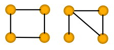
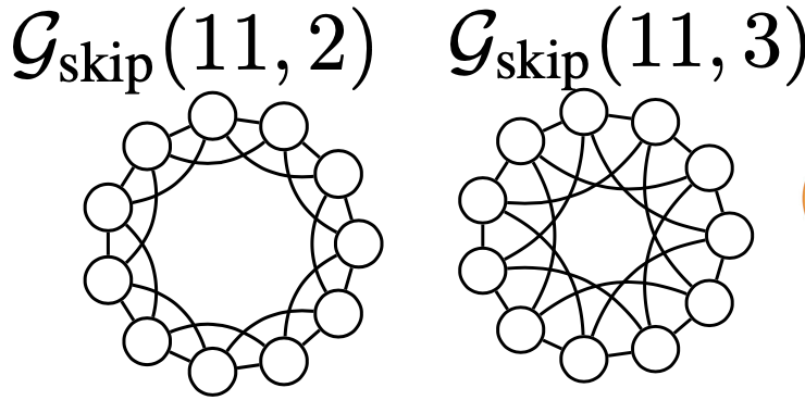
GINs have the same discriminative power as the WL graph isomorphism test (WL test is known to be capable of distinguishing most of real-world graph, except for some corner cases as on picture below; the prove of GINs relation to WL is in lecture).
GIN achieves state-of-the-art test performance in graph classification. GIN fits training data much better than GCN, GraphSAGE.
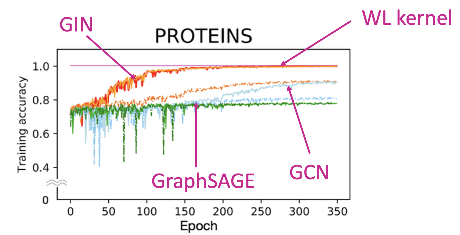
Same trend for training accuracy occurs across datasets. GIN outperforms existing GNNs also in terms of test accuracy because it can better capture graph structure.
Vulnerability of GNNs to noise in graph data
Probably, you’ve met examples of adversarial attacks on deep neural network where adding noise to image changes prediction labels.
Adversaries are very common in applications of graph neural networks as well, e.g., search engines, recommender systems, social networks, etc. These adversaries will exploit any exposed vulnerabilities.
To identify how GNNs are robust to adversarial attacks, consider an example of semi-supervised node classification using Graph Convolutional Neural Networks (GCN). Input is partially labeled attributed graph, goal is to predict labels of unlabeled nodes.
Classification Model contains two-step GCN message passing softmax ( Â ReLU (ÂXW(1))W(2). During training the model minimizes cross entropy loss on labeled data; during testing it applies the model to predict unlabeled data.
Attack possibilities for target node 𝑡 ∈ 𝑉 (the node whose classification label attack wants to change) and attacker nodes 𝑆 ⊂ 𝑉 (the nodes the attacker can modify):
- Direct attack (𝑆 = {𝑡})
- Modify the target‘s features (Change website content)
- Add connections to the target (Buy likes/ followers)
- Remove connections from the target (Unfollow untrusted users)
- Indirect attack (𝑡 ∉ 𝑆)
- Modify the attackers‘ features (Hijack friends of target)
- Add connections to the attackers (Create a link/ spam farm)
- Remove connections from the attackers (Create a link/ spam farm)
High level idea to formalize these attack possibilities: objective is to maximize the change of predicted labels of target node subject to limited noise in the graph. Mathematically, we need to find a modified graph that maximizes the change of predicted labels of target node: increase the loglikelihood of target node 𝑣 being predicted as 𝑐 and decrease the loglikelihood of target node 𝑣 being predicted as 𝑐 old.
In practice, we cannot exactly solve the optimization problem because graph modification is discrete (cannot use simple gradient descent to optimize) and inner loop involves expensive re-training of GCN.
Some heuristics have been proposed to efficiently obtain an approximate solution. For example: greedily choosing the step-by-step graph modification, simplifying GCN by removing ReLU activation (to work in closed form), etc (More details in Zügner+ KDD’2018).
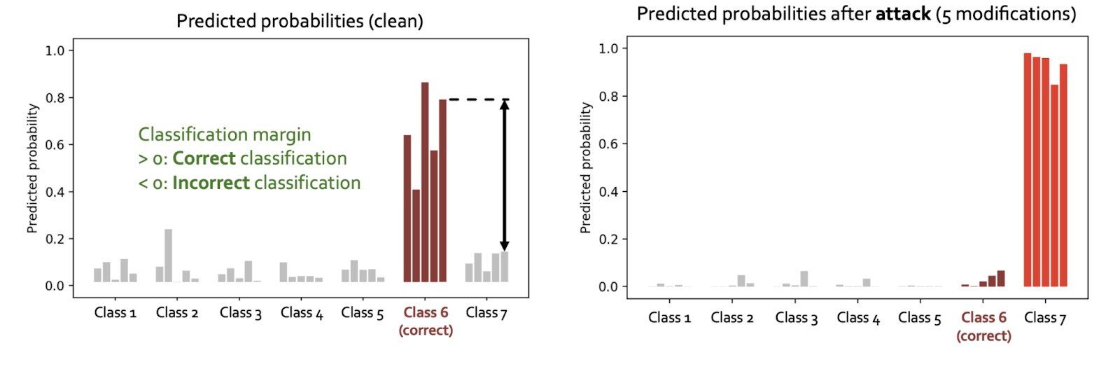
Attack experiments for semi-supervised node classification with GCN
Left plot below shows class predictions for a single node, produced by 5 GCNs with different random initializations. Right plot shows that GCN prediction is easily manipulated by only 5 modifications of graph structure (|V|=~2k, |E|=~5k).
Challenges of applying GNNs:
- Scarcity of labeled data: labels require expensive experiments -> Models overfit to small training datasets
- Out-of-distribution prediction: test examples are very different from training in scientific discovery -> Models typically perform poorly.
To partially solve this Hu et al. 2019 proposed Pre-train GNNs on relevant, easy to obtain graph data and then fine-tune for downstream tasks.
Lecture 19 – Applications of Graph Neural Networks
During this lecture, we describe 3 applications:
1. GNN recommendation (PinSage)
2. Heterogeneous GNN (Decagon)
3. Goal-directed generation (GCPN)
PinSage: GNN for recommender systems
In recommender systems, users interact with items (Watch movies, buy merchandise, listen to music) and the goal os to recommend items users might like:
- Customer X buys Metallica and Megadeth CDs.
- Customer Y buys Megadeth, the recommender system suggests Metallica as well.
From model perspective, the goal is to learn what items are related: for a given query item(s) Q, return a set of similar items that we recommend to the user.
Having a universal similarity function allows for many applications: Homefeed (endless feed of recommendations), Related pins (find most similar/related pins), Ads and shopping (use organic for the query and search the ads database).
Key problem: how do we define similarity:
1) Content-based: User and item features, in the form of images, text, categories, etc.
2) Graph-based: User-item interactions, in the form of graph/network structure. This is called collaborative filtering:
- For a given user X, find others who liked similar items.
- Estimate what X will like based on what similar others like.
Pinterest is a human-curated collection of pins. The pin is a visual bookmark someone has saved from the internet to a board they’ve created (image, text, link). The board is a collection of ideas (pins having something in common).
Pinterest has two sources of signal:
- Features: image and text of each pin
- Dynamic Graph: need to apply to new nodes without model retraining
Usually, recommendations are found via embeddings:
- Step 1: Efficiently learn embeddings for billions of pins (items, nodes) using neural networks.
- Step 2: Perform nearest neighbour query to recommend items in real-time.
PinSage is GNN which predicts whether two nodes in a graph are related.It generates embeddings for nodes (e.g., pins) in the Pinterest graph containing billions of objects. Key idea is to borrow information from nearby nodes simple set): e.g., bed rail Pin might look like a garden fence, but gates and rely adjacent in the graph.
Pin embeddings are essential in many different tasks. Aside from the “Related Pins” task, it can also be used in recommending related ads, home-feed recommendation, clustering users by their interests.
PinSage Pipeline:
- Collect billions of training pairs from logs.
- Positive pair: Two pins that are consecutively saved into the same board within a time interval (1 hour).
- Negative pair: random pair of 2 pins. With high probability the pins are not on the same board
- Train GNN to generate similar embeddings for training pairs. Train so that pins that are consecutively pinned have similar embeddings

where D is a set of training pairs from logs, zv is a “positive”/true example, zn is a “negative” example and Δ is a “margin” (how much larger positive pair similarity should be compared to negative).
3. Inference: Generate embeddings for all pins
4. Nearest neighbour search in embedding space to make recommendations.
Key innovations:
- On-the-fly graph convolutions:
- Sample the neighboUrhood around a node and dynamically construct a computation graph
- Perform a localized graph convolution around a particular node (At every iteration, only source node embeddings are computed)
- Does not need the entire graph during training
- Selecting neighbours via random walks
- Performing aggregation on all neighbours is infeasible: how to select the set of neighbours of a node to convolve over? Personalized PageRank can help with that.
- Define Importance pooling: define importance-based neighbourhoods by simulating random walks and selecting the neighbours with the highest visit counts.
- Choose nodes with top K visit counts
- Pool over the chosen nodes
- The chosen nodes are not necessarily neighbours.
- Compared to GraphSAGE mean pooling where the messages are averaged from direct neighbours, PinSAGE Importance pooling use the normalized counts as weights for weighted mean of messages from the top K nodes
- PinSAGE uses 𝐾 = 50. Performance gain for 𝐾 > 50 is negligible.
- Efficient MapReduce inference
- Problem: Many repeated computation if using localized graph convolution at inference step.
- Need to avoid repeated computation
- Introduce hard negative samples: force model to learn subtle distinctions between pins. Curriculum training on hard negatives starts with random negative examples and then provides harder negative examples over time. Obtain hard negatives using random walks:
- Use nodes with visit counts ranked at 1000-5000 as hard negatives
- Have something in common, but are not too similar
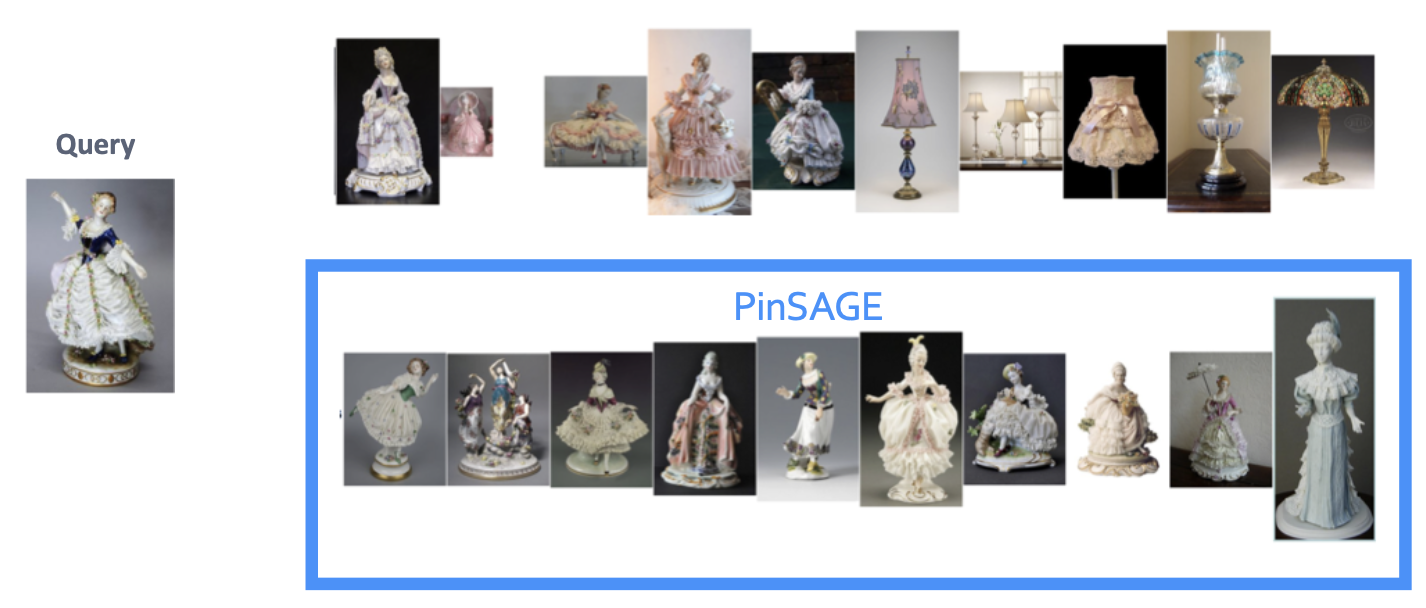
Experiments with PinSage
Related Pin recommendations: given a user just saved pin Q, predict what pin X are they going to save next. Setup: Embed 3B pins, find nearest neighbours of Q. Baseline embeddings:
- Visual: VGG visual embeddings.
- Annotation: Word2vec embeddings
- Combined: Concatenate embeddings

DECAGON: Heterogeneous GNN
So far we only applied GNNs to simple graphs. GNNs do not explicitly use node and edge type information. Real networks are often heterogeneous. How to use GNN for heterogeneous graphs?
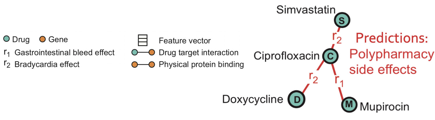
The problem we consider is polypharmacy (use of multiple drugs for a disease): how to predict side effects of drug combination? It is difficult to identify manually because it is rare, occurs only in a subset of patients and is not observed in clinical testing.
Problem formulation:
- How likely with a pair of drugs 𝑐, 𝑑 lead to side effect 𝑟?
- Graph: Molecules as heterogeneous (multimodal) graphs: graphs with different node types and/or edge types.
- Goal: given a partially observed graph, predict labeled edges between drug nodes. Or in query language: Given a drug pair 𝑐, 𝑑 how likely does an edge (𝑐 , r2 , 𝑑) exist?
Task description: predict labeled edges between drugs nodes, i.e., predict the likelihood that an edge (𝑐 , r2 , s) exists between drug nodes c and s (meaning that drug combination (c, s) leads to polypharmacy side effect r2.
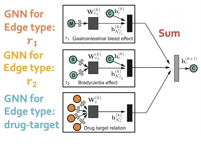
The model is heterogeneous GNN:
- Compute GNN messages from each edge type, then aggregate across different edge types.
- Input: heterogeneous graph.
- Output: node embeddings.
- During edge predictions, use pair of computed node embeddings.
- Input: Node embeddings of query drug pairs.
- Output: predicted edges.

Experiment Setup
- Data:
- Graph over Molecules: protein-protein interaction and drug target relationships.
- Graph over Population: Side effects of individual drugs, polypharmacy side effects of drug combinations.
- Setup:
- Construct a heterogeneous graph of all the data .
- Train: Fit a model to predict known associations of drug pairs and polypharmacy side effects.
- Test: Given a query drug pair, predict candidate polypharmacy side effects.
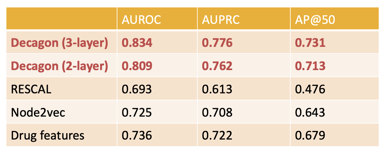
Decagon model showed up to 54% improvement over baselines. It is the first opportunity to computationally flag polypharmacy side effects for follow-up analyses.
GCPN: Goal-Directed Graph Generation (an extension of GraphRNN)
Recap Graph Generative Graphs: it generates a graph by generating a two level sequence (uses RNN to generate the sequences of nodes and edges). In other words, it imitates given graphs. But can we do graph generation in a more targeted way and in a more optimal way?
The paper [You et al., NeurIPS 2018] looks into Drug Discovery and poses the question: can we learn a model that can generate valid and realistic molecules with high value of a given chemical property?
Molecules are heterogeneous graphs with node types C, N, O, etc and edge types single bond, double bond, etc. (note: “H”s can be automatically inferred via chemical validity rules, thus are ignored in molecular graphs).
Authors proposes the model Graph Convolutional Policy Network which combines graph representation and Reinforcement Learning (RL):
- Graph Neural Network captures complex structural information, and enables validity check in each state transition (Valid).
- Reinforcement learning optimizes intermediate/final rewards (High scores).
- Adversarial training imitates examples in given datasets (Realistic).
Steps of GCPN and shown on the picture below:
- (a) Insert nodes/scaffolds.
- (b) Compute state via GCN.
- (c) Sample next action.
- (d) Take action (check chemical validity).
- (e, f) Compute reward.

To set the reward in RL part:
- Learn to take valid action: at each step, assign small positive reward for valid action.
- Optimize desired properties: at the end, assign positive reward for high desired property.
- Generate realistic graphs: at the end, adversarially train a GCN discriminator, compute adversarial rewards that encourage realistic molecule graphs
Reward rt is final reward (domain-specific reward) and step reward (step-wise validity reward).
Training consists of two parts:
- Supervised training: train policy by imitating the action given by real observed graphs. Use gradient.
- RL training: train policy to optimize rewards. Use standard policy gradient algorithm.

GCPN can perform different tasks:
- Property optimization: generate molecules with high specified property score.
- Property targeting: generate molecules whose specified property score falls within given range.
- Constrained property optimization: edit a given molecule for a few steps to achieve higher specified property score.
